Basics of Multiple Regression and Underlying Assumptions
Use of Multiple Linear Regression
- Identify relationships between variables
- Example: understand how returns are influenced by a set of underlying factors.
- Test existing theories
- Example: the explanatory power of the CAPM model.
- Forecast
- Example: using financial data to predict the probability of default.
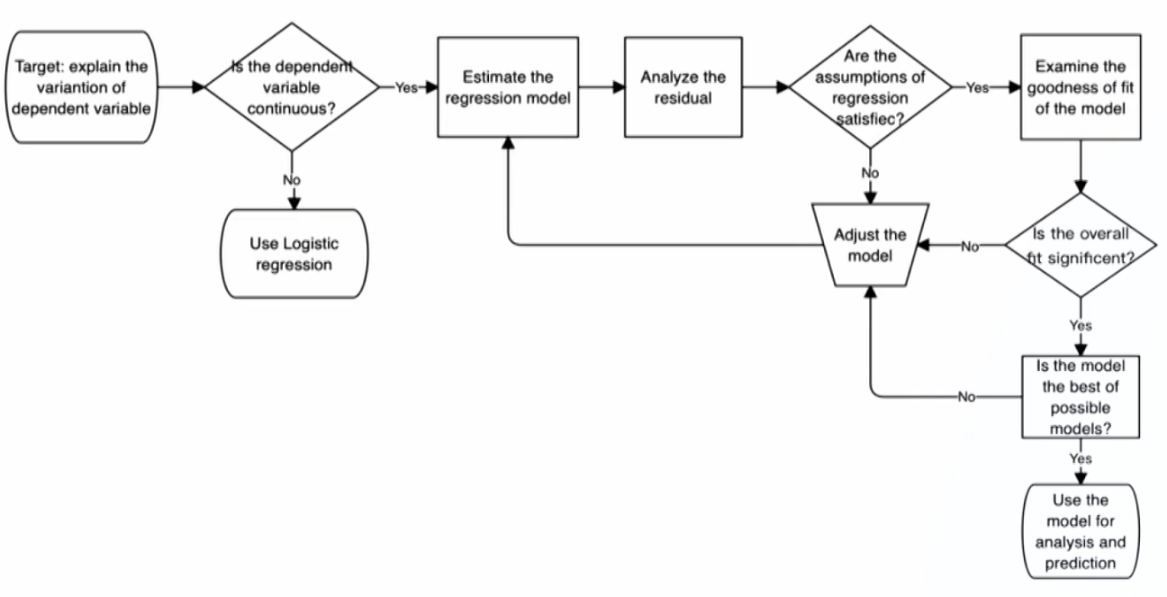
Regression Process
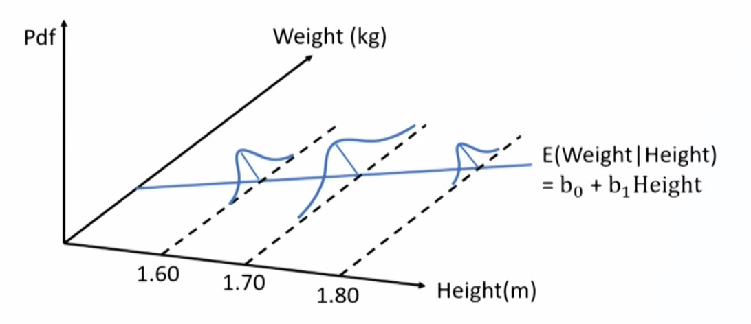
Multiple linear regression model
\mathrm{Y}_{\mathrm{i}}=\mathrm{b}_0+\mathrm{b}_1\mathrm{X}_{1\mathrm{i}}+\mathrm{b}_2\mathrm{X}_{2\mathrm{i}}+\cdots+\mathrm{b}_{\mathrm{k}} \mathrm{X}_{\mathrm{ki}}+\varepsilon_{\mathrm{i}}- Intercept term (b_0)
- The value of the dependent variable when the independent variables are all equal to zero.
- Slope coefficient (b_j)
- The expected increase in the dependent variable for a 1-unit increase in that independent variable, holding the other independent variables constant.
- Also called partial slope coefficients.
Assumptions of multiple linear regression model
- Linearity: the relationship between the dependent variable (Y) and the independent variable (X) is linear.
- Test linearity: scatter plot of the dependent variable versus one independent variable.
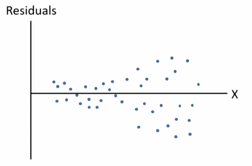
- Homoskedasticity: the variance of the error term is the same for all observations.
- Test homoskedasticity of error term: scatter plot of the residual versus dependent variable or independent variable.
- Normality: the error term is normally distributed.
- Test normality of error term: normal QQ plot of the residual
- Independence: The error term is uncorrelated across observations; No exact linear relation between independent variables.
- Test independence of error term: scatter plot of the residual versus dependent variable or independent variable.
- Test independence of independent variables: scatter plot of one independent variable versus another independent variable.
- The independent variables are not random
Evaluating Regression Model Fit and Interpreting Model Results
Goodness of Fit拟合优度
ANOVA analysis
- ANOVA table for multiple linear regression:
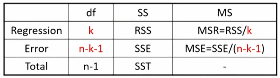
- Standard error of estimate: \mathrm{SEE}=\sqrt{\mathrm{MSE}}
- F=\mathrm{MSR} / \mathrm{MSE} with df of k and n-k-1
- R^2=\mathrm{ RSS } / \mathrm{SST}
R2(coefficient of determination)
\mathrm{R}^2=\frac{\text { Explained variation }}{\text { Total variation }}=\frac{\mathrm{RSS}}{\mathrm{SST}}=\frac{\mathrm{SST}-\mathrm{SSE}}{\mathrm{SST}}- Test the overall effectiveness (goodness of fit) of the entire set of independent variables (regression model) in explaining the dependent variable.
- E.g., an \mathrm{R}^2 of 0.7 indicates that the model, as a whole,explains 70% of the variation in the dependent variable.
- For multiple regression, however, \mathrm{R}^2 will increase simply by adding independent variables that explain even a slight amount of the previously unexplained variation.
- Even if the added independent variable is not statistically significant, \mathrm{R}^2 will increase.
- Models that aim for high \mathrm{R}^2 will lead to overfitting problem.
Adjusted R2(\overline{\mathrm{R}}^2)
\overline{\mathrm{R}}^2=1-\left[\left(\frac{\mathrm{n}-1}{\mathrm{n}-\mathrm{k}-1}\right) \times\left(1-\mathrm{R}^2\right)\right]- \overline{\mathrm{R}}^2\le \mathrm{R}^2 and may less than zero, if \mathrm{R}^2 is low enough or the independent variables is too many.
- Adding a new independent variable may either increase or decrease the \overline{\mathrm{R}}^2.
- If the value of \overline{\mathrm{R}}^2 increase, the new independent variable should be added.
AIC(Akaike's information criterion)
\mathrm{AIC}=\mathrm{n} \times \ln \left(\frac{\mathrm{SSE}}{\mathrm{n}}\right)+2(\mathrm{k}+1)- The lower the better.
- 2(k + 1) is the penalty for adding independent variable.
- Measure of model parsimony简洁性.
BIC(Schwarz's Bayesian information criterion)
\mathrm{BIC}=\mathrm{n} \times \ln \left(\frac{\mathrm{SSE}}{\mathrm{n}}\right)+\ln (\mathrm{n})(\mathrm{k}+1)- Compared to AIC, BIC assesses a greater penalty for adding independent variables.
- In practice, AIC is preferred for prediction while BIC is more likely to be used for seeking best fitness
Hypotheses Testing and Prediction
Hypothesis testing for regression coefficient
- To test whether an independent variable explains the variation in the dependent variable
H_0: b_j=0; H_a: b_j \neq0; - Test statistic:
\mathrm{t}=\frac{\hat{{b}_1}}{\mathrm{s}_{\hat{{b}_1}}} - Decision rule: reject \mathrm{H}_0 if |\mathrm{t}|\gt \mathrm{t}_{\text {critical }} or p-value <significance level (\alpha)
- Rejection of \mathrm{H}_0 means the slope coefficient is significantly different from zero.
F-test
- Test whether the independent variables, as a group, help explain the dependent variable; or assess the effectiveness of the model, as a whole, in explaining the dependent variable.
H_0: b_1=b_2=b_3=\ldots=b_k=0; H_a: \exists b_j\neq 0 - Test statistic:
\mathrm{F}=\frac{\mathrm{MSR}}{\mathrm{MSE}}=\frac{\mathrm{RSS}/k}{\mathrm{SSE}/(n-k-1)}\sim F(k,n-k-1) - Decision rule: reject \mathrm{H}_0 if \mathrm{F} \gt \mathrm{F}_{\text {critical }} or p-value <significance level (\alpha)
- Rejection of Ho means there is at least one regression coefficient is significantly different from zero, thus at least one independent variable makes a significant contribution to the explanation of dependent variable.
- Restricted model (nested model) is nested within the unrestricted model.
\mathrm{Y}_{\mathrm{i}}=\mathrm{b}_0+\mathrm{b}_1\mathrm{X}_{1\mathrm{i}}+\mathrm{b}_2\mathrm{X}_{2\mathrm{i}}+\varepsilon_{\mathrm{i}}- To test whether b_3=b_4=0.
- The number of restrictions is denoted as q.
- The comparison of models implies a null hypothesis that involves a joint restriction on two coefficients.
H_0: b_3=b_4=0\quad H_a: \exists b_j \neq0(j=3,4) - Test statistic:
\mathrm{F}=\frac{( \mathrm{SSE}_{\text{restricted}} - \mathrm{SSE}_{\text{unrestricted}} ) /q }{\mathrm{SSE}_{\text{unrestricted}} /(n-k-1)}\sim F(q,n-k-1)
Model Misspecification
Definition of Misspecification
Definition and effects of model misspecification
- The set of variables and functional form are not appropriate,leading to
- Biased and inconsistent regression coefficients
- Unreliable hypothesis testing
- Inaccurate predictions.
- Misspecified functional form
- Omitted variables(遗漏变量,依赖与已有的自变量有关或无关的变量)
- Inappropriate form of variables(错误的变量形式,比如不是实际上是对数线性的)
- Inappropriate variable scaling(未使用缩放的数据,数据数量级差距太大)
- Inappropriate data pooling(错误融合来自不同总体的数据)
Avoiding model misspecification
- The model should be grounded in cogent economic reasoning.
- The model should be parsimonious.
- The model should be examined for violations of regression assumptions before being accepted.
- The model should be formed appropriately.
- The model should be tested and be found useful out of sample before being accepted.
Violations of Regression Assumptions
Heteroskedasticity
- The variance of error terms differs across observations.
- Graphic illustration of heteroskedasticity in simple linear regression:
- Graphic illustration of heteroskedasticity in simple linear regression:
- Types of heteroscedasticity
- Unconditional heteroskedasticity: heteroskedasticity of the error variance is not correlated with the independent variables方差变化是随机的. Creates no major problems for statistical inference.
- Conditional heteroskedasticity: heteroskedasticity of the error variance is correlated with (conditional on) the values of the independent variables方差变化与自变量相关. Does create significant problems for statistical inference.
- Effects of heteroskedasticity
- The coefficient estimates (\hat{b}_j) aren't affected.估计方向正确
- The standard errors of coefficient (s_{\hat{b}_j})are usually unreliable.
With financial data, s_{\hat{b}_j} are most likely underestimated 估计范围过于精确
The t-statistics will be inflated 检验量变大
Tend to find significant relationships where none actually exist (type I error) 容易认为模型有效 - The F-test is also unreliable.
- Testing for conditional heteroskedasticity
- Examining scatter plots of the residuals.
- Breusch-Pagen \chi^2 test 二次回归看是否有相关性,越大越拒绝

- Examining scatter plots of the residuals.
- Correcting for heteroskedasticity
- Use robust standard errors to recalculate the t-statistics. Also called White-corrected standard errors. 用放大的标准误
- Use generalized least squares, other than ordinary least squares, to build the regression model. 用广义最小二乘法
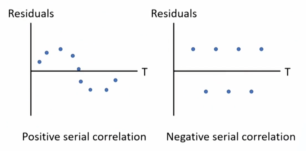
Serial correlation
- The error terms are correlated with one another, and typically arises in time-series regressions.
- Positive serial correlation: a positive/negative error for one observation increases the chance of a positive/negative error for another observation 动量效应.(More often)
- Negative serial correlation: a positive/negative error for one observation increases the chance of a negative/positive error for another observation 反转效应.
- Effects of serial correlation
- The coefficient estimates aren't affected.估计方向正确
- The standard errors of coefficient are usually unreliable.
Positive serial correlation: standard errors underestimated and t-statistics inflated, suggesting significance when there is none (type I error);估计范围过于精确,后果类似异方差
Negative serial correlation: vice versa (type II error). 估计范围过于宽泛,与异方差后果完全相反 - The F-test is also unreliable.
- Testing for serial correlation
- Examining scatter plots of the residuals.
- The Durbin-Watson (DW) test, Limited for detecting first-order serial correlation一阶自相关.
结果0-4, 0正相关、4负相关、2不相关 - The Breusch-Godfrey (BG) test 二次回归看滞后项系数是否为0
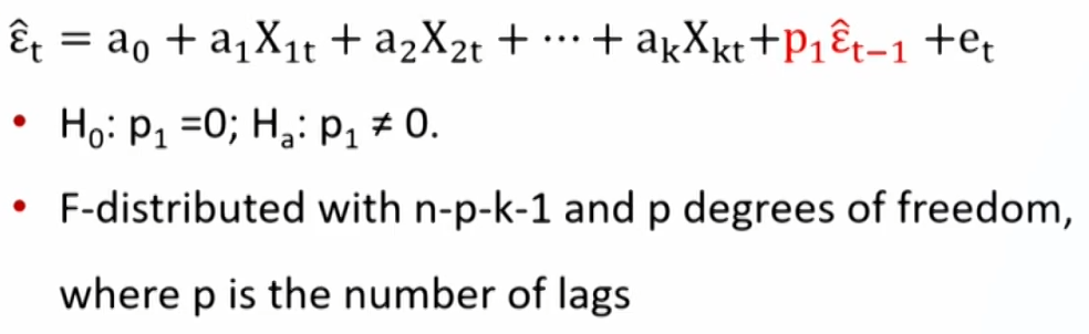
- Examining scatter plots of the residuals.
- Correcting for serial correlation
- Adjust the coefficient standard errors (recommended). 用放大的标准误
Serial-correlation consistent standard errors
Adjusted standard errors
Newey-West standard errors 既能解决序列自相关,又能解决条件异方差
Robust standard errors.
Also correct for conditional heteroskedasticity. - Modify the regression equation itself. 将模型引入滞后项
- Adjust the coefficient standard errors (recommended). 用放大的标准误
Multicollinearity
- Two or more independent variables (or combinations of independent variables) are highly (but not perfectly) correlated with each other.
- Effects of multicollinearity
- Estimates of regression coefficients become extremely imprecise and unreliable. 估计方向错误
- Standard errors of coefficients inflated 估计范围过于宽泛,类似负的序列自相关
- t-statistics underestimated. 估计值变小
- Tend to neglect significant relationships when there actually exist (type II error). 容易认为模型无效
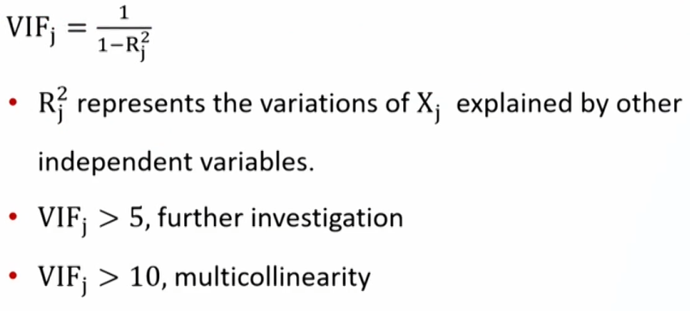
- Testing for multicollinearity
- Classica Methods: The t-tests indicate that none of the regression coefficients is significant, while R2 is high and F-test indicates overall significance. 单独看没有显著性, 放一起却显著
- VIF (variance inflation factor), 拿自变量j和剩下的自变量做回归
- Correcting for multicollinearity
- Excluding one or more of the correlated independent variables.
- Using a different proxy for one of the variables 找替代变量
- Increasing the sample size. 避免偶然因素
- 遗漏变量与多重共线性
- 有一点共线性但忽视:遗漏变量
- 有很大共线性但引入:多重共线性
Extensions of Multiple Regression
Influence Analysis
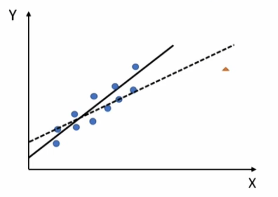
- Regression results can be biased by a small number of observations in a sample.
- An influential observation is an observation whose inclusion may significantly alter regression results.
- High-leverage point
- An extreme value of independent variable.
- Leverage (\mathrm{h}_{ii}) measures the distance between the value of the ith observation and the mean value of all n observations.
- Between 0 and 1, the higher, the more influence the ith observation.
- Rule of thumb临界值: exceeds \frac{3(k+1)}{n} potentially influential observation.
- An extreme value of independent variable.
- Outlier
- An extreme value of dependent variable.
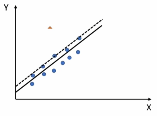
- Studentized residual (\mathrm{t}_{i^\ast}) Compare the observed Y values (on n observations) with the predicted Y values resulting from the models with the ith observation deleted (on n-1 observations),with degree of freedom n-k-2
- Rule of thumb: |\mathrm{t}|\gt \mathrm{t}_{\text {critical }}, potentially influential observation.
- An extreme value of dependent variable.
- Cook's Distance(Cook's D)
\mathrm{D}_{\mathrm{i}}=\frac{\mathrm{e}_{\mathrm{i}}^2}{\mathrm{k} \times \mathrm{MSE}}\left[\frac{\mathrm{h}_{\mathrm{ii}}}{\left(1-\mathrm{h}_{\mathrm{ii}}\right)^2}\right]- depends on both residuals and leverages.
- A large \mathrm{D}; indicates that the ith observation strongly influences the regression's estimated values.
- Rule of thumb: exceed 0.5,1.0,or 2\sqrt{k/n}, potentially influential
Qualitative Variables
Qualitative independent variables
- Financial analysts often need to use qualitative variables as independent variables in a regression.
- Qualitative variable定性指标: nominal定类 type or ordinal定序 type variable. E.g., gender, education.
Dummy variable
- Dummy variable(indicator variable) can be used to represent qualitative variables in regression analysis.
- Dummy variable: qualitative variable with value of "0" or "1".
- If we want to distinguish among n categories, we need n-1 dummy variables.
- The category not assigned becomes the "base" or "control" group.
- Example: use dummy variables to analyze the annual income for CFA exam participants.
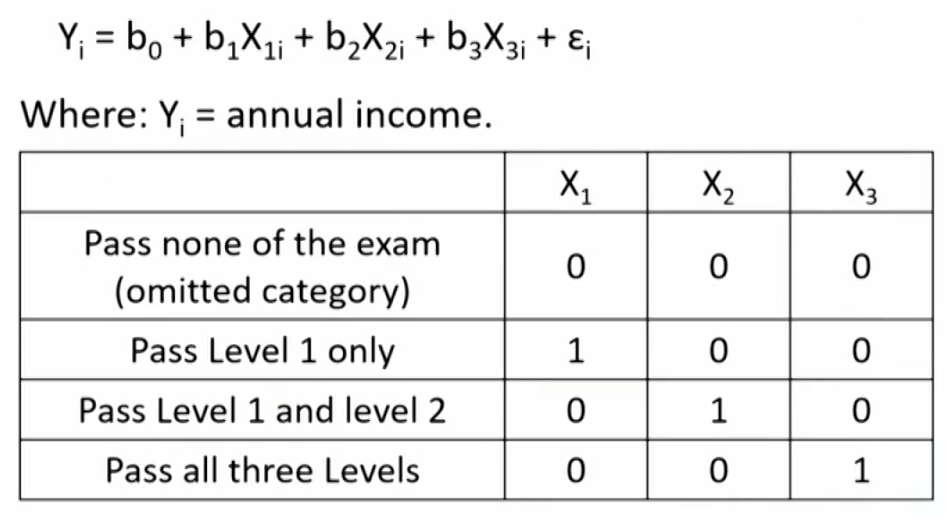
- Interpretation of regression coefficient
- Intercept coefficient (b_0): the average value of dependent variable for the omitted category.
- Slope coefficient (b_j): the difference in dependent variable (on average) between the category represented by the dummy variable and the omitted category.
- Individual t-tests on the dummy variable coefficients indicate whether the difference is significant.
- Interpreting Dummy Variables
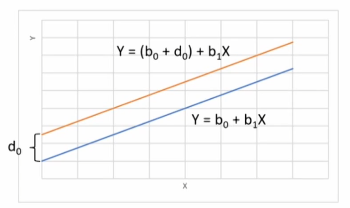 Y=b_0+d_0D+b_1X+\varepsilon
- if D=0, Y=b_0+b_1X+\varepsilon
- if D=1, Y=(b_0+d_0)+b_1X+\varepsilon
- Slope dummy Variables
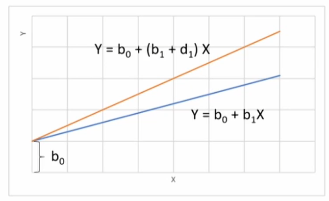 Y=b_0+b_1X+d_1(D \cdot X)+\varepsilon
- if D=0, Y=b_0+b_1X+\varepsilon
- if D=1, Y=b_0+(b_1+d_1)X+\varepsilon
Qualitative dependent variable
- Dummy variables can also be used as dependent variables in regression analysis.
- Logistic transformation → Logit model
- A logit model:
\ln \left(\frac{\mathrm{p}}{1-\mathrm{p}}\right)=\mathrm{b}_0+\mathrm{b}_1\mathrm{X}_1+\mathrm{b}_2\mathrm{X}_2+\mathrm{b}_3\mathrm{X}_3+\varepsilon- \ln \left(\frac{\mathrm{p}}{1-\mathrm{p}}\right) is known as log odds or logit function
- The event probability
\mathrm{p}=\frac{1}{1+e^{-\left(\mathrm{b}_0+\mathrm{b}_1\mathrm{X}_1+\mathrm{b}_2\mathrm{X}_2+\mathrm{b}_3\mathrm{X}_3\right)}}
- Fit of logit model
- Coefficients are typically estimated using the maximum likelihood estimation (MLE).
- Ajusted R2 is not suitable, use Pseudo R2
- Log likelihood metric is always negative, so higher values(closer to 0) indicate a better fitting model.
- Likelihood ratio (LR) test: is similar to the joint F-test
For example: to test whether b_3=b_4=0
LR =-2(Log likelihood restricted model -Log likelihood unrestricted model). 越大越拒绝
Time-Series Analysis
Trend Models
- Linear trend models
 \mathrm{y}_{\mathrm{t}}=\mathrm{b}_0+\mathrm{b}_1\mathrm{t}+\varepsilon_{\mathrm{t}} \quad \hat{\mathrm{y}}=\hat{\mathrm{b}}_0+\hat{\mathrm{b}}_1\mathrm{t}
- Work well in fitting time series that have constant change amount with time.
- Log-linear trend models
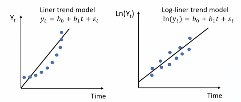 \mathrm{y}_{\mathrm{t}}=\mathrm{e}^{\left(\mathrm{b}_0+\mathrm{b}_1\mathrm{t}+\varepsilon_{\mathrm{t}}\right)} \quad \operatorname{Ln}\left(\mathrm{y}_{\mathrm{t}}\right)=\mathrm{b}_0+\mathrm{b}_1\mathrm{t}+\varepsilon_{\mathrm{t}}
- Work well in fitting time series that have constant growth rate with time (exponential growth).
- Linear trend model vs. Log-linear trend model
- If data plots with a linear shape (constant change amount), a linear trend model may be appropriate.
- If data plots with a non-linear (curved) shape (constant growth rate), a log-linear model may be more suitable.
- Limitations of trend models
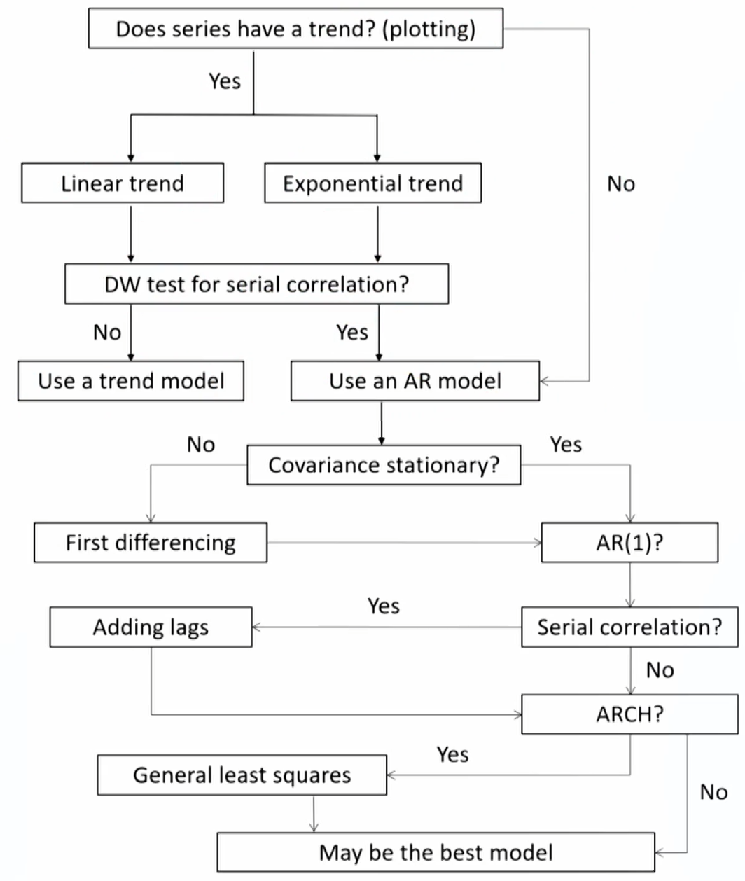
- The trend model is not appropriate for time series when data exhibit serial correlation. 残差自相关
- Use the Durbin-Watson statistic to detect serial correlation. Test whether the first autocorrelations (\rho_{\varepsilon_{\mathrm{t}}, \varepsilon_{\mathrm{t}-1}}) of the residual equals to zero.
Autoregressive Models
- Autoregressive model: use the past values of dependent variable as independent variables.
- AR(1): First-order autoregressive model
\mathrm{x}_{\mathrm{t}}=\mathrm{b}_0+\mathrm{b}_1\mathrm{x}_{\mathrm{t}-1}+\varepsilon_{\mathrm{t}} - AR(p): p-order autoregressive model
\mathrm{x}_{\mathrm{t}}=\mathrm{b}_0+\mathrm{b}_1\mathrm{x}_{\mathrm{t}-1}+\mathrm{b}_2\mathrm{x}_{\mathrm{t}-2}+\ldots+\mathrm{b}_{\mathrm{p}} \mathrm{x}_{\mathrm{t}-\mathrm{p}}+\varepsilon_{\mathrm{t}}
- AR(1): First-order autoregressive model
- Covariance stationary协方差平稳 is a key assumption for AR model to be valid based on ordinary least squares (OLS) estimates, and must satisfy three principal requirements:
- Constant and finite expected value in all periods.
- Constant and finite variance in all periods.
- Constant and finite covariance with itself for a fixed number of periods in the past or future in all periods.
- Detecting serial autocorrelation
- Step 1: Estimate the AR(k) model using linear regression
- Step 2: Compute the autocorrelations (\rho_{\varepsilon_t, \varepsilon_{t-k}}) of the residual, The order of the correlation is given by k, where k represents the number of periods lagged.
- Step 3: Test if the autocorrelations are significantly different from zero.
\mathrm{t}=\frac{\hat{\rho}_{\varepsilon_{\mathrm{t}}, \varepsilon_{\mathrm{t}-\mathrm{k}}}}{1/ \sqrt{\mathrm{T}}}\sim t(T-2)
If the residual autocorrelations differ significantly from 0, the model is not correctly specified and need to be modified.
Moving-Average Models
- Moving-average (MA) Models
- MA(1): First-order moving-average model
x_t=\varepsilon_t+\theta \varepsilon_{t-1} - MA(q): q-order moving-average model
x_t=\varepsilon_t+\theta_1\varepsilon_{t-1}+\cdots+\theta_q \varepsilon_{t-q}
- MA(1): First-order moving-average model
- How can we tell which types of model may fit a time series better? We examine the autocorrelations.
- For an MA(q) model, the first q autocorrelations will be significantly different from 0, and all autocorrelations beyond that will be equal to 0.
- For an AR model, the autocorrelations of most autoregressive time series start large and decline gradually.
- ARMA model
- ARMA(p,q):AR(p)modeland MA(q)model iscombined
\mathrm{y}_t=b_0+b_1y_{t-1}+\cdots+b_p y_{t-p}+\varepsilon_t+\theta_1\varepsilon_{t-1}+\cdots+\theta_q \varepsilon_{t-q} - Limitations
Sensitive to inputs.
Choosing the right ARMA model is an art.
- ARMA(p,q):AR(p)modeland MA(q)model iscombined
Violation of Assumptions
Seasonality
- Seasonality: time series that shows regular patterns of movement within the year.
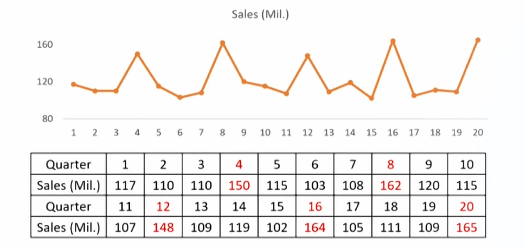
- Testing of seasonality: test if the seasonal autocorrelation of the residual will differ significantly from O.
- The 4th autocorrelation in case of quarterly data: \rho_{\varepsilon_{t},\varepsilon_{t-4m}}.
- The 12th autocorrelation in case of monthly data: \rho_{\varepsilon_{t},\varepsilon_{t-12m}}.
- Modeling seasonality: include a seasonal lag in AR model:
- Quarterly data: \mathrm{x}_{\mathrm{t}}=\mathrm{b}_0+\mathrm{b}_1\mathrm{x}_{\mathrm{t}-1}+\mathrm{b}_2\mathrm{x}_{\mathrm{t}-4}+\varepsilon_{\mathrm{t}}
- Monthly data: \mathrm{x}_{\mathrm{t}}=\mathrm{b}_0+\mathrm{b}_1\mathrm{x}_{\mathrm{t}-1}+\mathrm{b}_2\mathrm{x}_{\mathrm{t}-12}+\varepsilon_{\mathrm{t}}
Unit Root
- Mean reversion
- A time series shows mean reversion if it has a tendency to move towards its mean.
- Tends to fall when it is above its mean and rise when it is below its mean.
- Mean-reverting level for an AR(1) model:
\mathrm{x}_{\mathrm{t}}=\frac{\mathrm{b}_0}{1-\mathrm{b}_1}- |b_1|\lt 1 in AR(1) model → finite mean-reverting level.
- Covariance stationary → finite mean-reverting level.
- Simple random walk: time series in which the value of the series in one period is the value of the series in the previous period plus an unpredictable random error.
\mathrm{x}_{\mathrm{t}}=\mathrm{x}_{\mathrm{t}-1}+\varepsilon_{\mathrm{t}}- A special AR(1) model with b_0=0 and b_1=1
- The best forecast of \mathrm{x}_\mathrm{t} is \mathrm{x_{\mathrm{t}-1}}
- Random walk with a drift: a random walk with the intercept term that not equal to zero (bo ≠ 0).
\mathrm{x}_{\mathrm{t}}=\mathrm{b}_0+\mathrm{x}_{\mathrm{t}-1}+\varepsilon_{\mathrm{t}}- Increase or decrease by a constant amount (\mathrm{b}_0) in each period.
- Random walk vs. covariance stationary
- A random walk will not exhibit covariance stationary.
A time series must have a finite mean reverting level to be covariance stationary.
A random walk has an undefined mean reverting level.
\mathrm{x}_{\mathrm{t}}=\frac{\mathrm{b}_0}{1-\mathrm{b}_1}=\frac{0}{0} - The least squares regression method doesn't work to estimate an AR(1) model on a time series that is actually a random walk.
- A random walk will not exhibit covariance stationary.
- Unit root
- The time series is said to have a unit root if the lag coefficient is equal to one (b_1=1) and will follow a random walk process.
- Testing for unit root can be used to test for non-stationarity since a random walk is not covariance stationary.
- But t-test for b_1=1 in AR model is invalid to test unit root. t-test不可靠
- Dickey-Fuller test for unit root
- Based on the AR(1) model: \mathrm{x}_t=\mathrm b_0+\mathrm b_1\mathrm{x}_{\mathrm t-1}+\varepsilon_t
- Subtract \mathrm{x}_{\mathrm{t}-1} from both sides: \mathrm{x}_{\mathrm{t}}-\mathrm{x}_{\mathrm{t}-1}=\mathrm{b}_0+\left(\mathrm{b}_1-1\right) \mathrm{x}_{\mathrm{t}-1}+\varepsilon_{\mathrm{t}}
Or: \mathrm{x}_{\mathrm{t}}-\mathrm{x}_{\mathrm{t}-1}=\mathrm{b}_0+\mathrm{g}_1\mathrm{x}_{\mathrm{t}-1}+\varepsilon_{\mathrm{t}}, where: \mathrm{g}_1=\mathrm{b}_1-1 - \mathrm{H}_0: \mathrm{g}_1=0; \mathrm{H}_{\mathrm{a}}: \mathrm{g}_1\lt 0。
Calculate t-statistic and use revised critical values比传统的t经验值大一点
If fail to reject \mathrm{H}_0, there is a unit root and the time series is non-stationary
- First differencing
- A random walk can be transformed to a covariance stationary time series by first differencing.
\mathrm y_{\mathrm t}=\mathrm x_{\mathrm t}-\mathrm x_{\mathrm t-1}\rightarrow \mathrm y_{\mathrm t}=\varepsilon_t - Then, \mathrm y_{\mathrm t} is covariance stationary variable with a finite mean-reverting level of 0/(1-0)=0
- A random walk can be transformed to a covariance stationary time series by first differencing.
Heteroskedasticity
- Autoregressive Conditional Heteroskedasticity(ARCH)
- Conditional heteroskedasticity: heteroskedasticity of the error variance is correlated with (conditional on) the values of the independent variables.
- ARCH: conditional heteroskedasticity in AR models. When ARCH exists, the standard errors of the regression coefficients in AR models are incorrect, and the hypothesis tests of these coefficients are invalid.
- ARCH model and GARCH model 残差的方差不固定,额外进行建模
- Variance of the error in a particular time-series model in one period depends on how large the squared error was in the previous period.
\sigma_t^2=\mathrm{a}_0+\mathrm{a}_1\varepsilon_{t-1}^2+\mathrm{u}_{\mathrm{t}} - In an ARCH(p) model, the variance of the error term in the current period depends linearly on the squared errors from the previous p periods:
\sigma_t^2=\mathrm{a}_0+\mathrm{a}_1\varepsilon_{t-1}^2+\cdots+\mathrm{a}_{\mathrm{p}} \varepsilon_{t-p}^2+\mathrm{u}_{\mathrm{t}}
- Variance of the error in a particular time-series model in one period depends on how large the squared error was in the previous period.
- Detecting conditional heteroskedasticity
- Run a regression of \hat{\varepsilon}_t^2=a_0+a_1\hat{\varepsilon}_{\mathrm{t}-1}^2+u_t
- If the coefficient a_1 is statistically significantly different from 0, the time series has conditional heteroskedasticity problem.
- If a time series model has conditional heteroskedasticity problem, generalized least squares must be used.
- Predicting variance with ARCH models
\hat{\sigma}_{\mathrm{t}+1}^2=\hat{\mathrm{a}}_0+\hat{\mathrm{a}}_1\hat{\varepsilon}_{\mathrm{t}}^2- If a time-series model has ARCH(1) errors, the ARCH model can be used to predict the variance of the residuals in future periods.
More than one time series
- When running regression with two time series, either or both could be subject to non-stationarity

- Dickey-Fuller tests can be used to detect unit root:
- If none of the time series has a unit root, linear regression can be safely used.
- Only one time series has a unit root, linear regression can not be used.
- Cointegration协整: two time series have long-term financial or economic relationship so that they do not diverge from each other without bound in the long run. 相互牵制
- If both time series have a unit root, then
- If the two series are cointegrated, linear regression can be used.
- If the two series are not cointegrated, linear regression can not be used.
- Engle and Granger test for cointegration
- Step 1: x_{1,t}=b_0+b_1x_{2,t}+\varepsilon_t
- Step 2: test whether the error term from the regression has a unit root using a Dickey-Fuller test.
Use the critical values computed by Engle and Granger. - Step 3: make the decision
Error term has unit root → not cointegrated
Error term has no unit root → cointegrated
Model Selection
- Steps in time series forecasting
- Comparing forecasting model performance
- In-sample forecasts errors: the residuals within sample period to estimate the model.
- Out-of-sample forecasts errors: the residuals outside sample period to estimate the model.
- Root mean squared error (RMSE) criterion: the model with the smallest RMSE for the out-of-sample data is typically judged most accurate.
- Instability of regression coefficients
- Financial and economic relationships are inherently dynamic,so the estimates of regression coefficients of the time-series model can change substantially across different sample periods.
- There is a tradeoff between reliability and stability. Models estimated with shorter time series are usually more stable but less reliable.
Machine Learning
Introduction of Machine Learning
Machine learning (ML)
- Machine learning comprises diverse approaches by which computers are programmed to improve performance in specified tasks with experience.
- Find the pattern, apply the pattern.
- Based on large amounts of data.
- Less restribitons compared to statistical approaches.
- Machine learning techniques are better able than statistical approaches to handle problems with many variables (high dimensionality) or with a high degree of non-linearity.
- Machine learning has theoretical and practical implications for investment management, from client profiling, to asset allocation, to stock selection, to portfolio construction and risk management, to trading
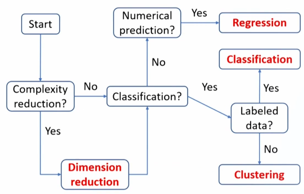
Types of machine learning
- Machine learning is broadly divided into three distinct classes of techniques:
- Supervised learning
- Unsupervised learning
- Deeplearning/ reinforcement learning
- Supervised learning infers patterns between a set of inputs(the X's) and the desired output (Y), the inferred pattern is then used to predict output given an input set
- Supervised learning requires a labeled data set, containing matched sets of observed inputs and the associated output.
- Using this data set to infer the pattern between the inputs and output is called "training" the algorithm.
- Based on the nature of the target (Y) variable, supervised learning can be divided into two categories of problems:
Regression problems: the target variable is continuous.
Classification problems: the target variable is categorical or ordinal.
- Unsupervised learning does not make use of labeled data.
- We have inputs (X's) that are used for analysis without any target (Y) being supplied.
- Unsupervised learning algorithms seek to discover structure within the data themselves.
- Two important types of problems are well suited to unsupervised learning:
Dimension reduction(降维): reduce the number of features while retaining variation across observations to preserve the information contained in that variation.
Clustering(聚类): focus on sort observations into groups(clusters), such that observations in the same cluster are more similar to each other.
- Deep learning and reinforcement learning
- Both deep learning and reinforcement learning can be either supervised or unsupervised, and are based on neural networks (NNs, 神经网络), NNs are also called artificial neural networks (ANNs).
- Neural networks consist of nodes (neurons, 神经元) connected by links, and have three types of layers: an input layer, hidden layers, and an output layer.
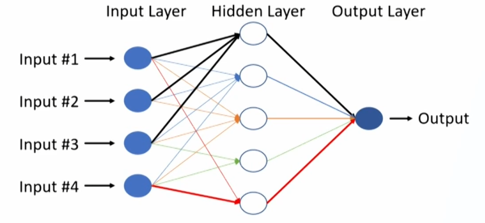
Neurons: any of the nodes to the right of the input layer.
Summation operator: multiplies each value by its respective weight and then sums the weighted values to form the total net input.
Activation function: transforms the total net input into the final output of the node.
Forward propagation vs. backward propagation - Deep learning nets(DLNs) can address highly complex tasks, such as image classification, face recognition, speech recognition, and natural language processing.
Deep neural networks (DNNs): neural networks with many hidden layers (at least 3 but often more than 20 hidden layers). - Reinforcement learning. In reinforcement learning, a computer learns from interactingwith itself (or data generated by the same algorithm).
Unlike supervised learning, reinforcement learning has neither direct labeled data nor instantaneous feedback.
The algorithm needs to observe its environment, learn by testing new actions, and reuse its previous experiences.
Determination of problems
Evaluating Algorithm Performance
Division of data set
- The whole data set can typically be divided into three non-overlapping samples:
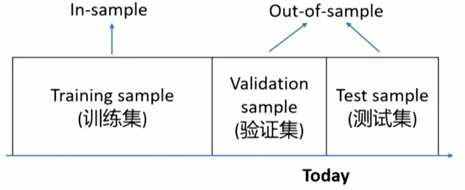
- Training sample: train the model. Often referred to as being "in-sample".
- Validation sample: validate and tune the model.
- Test sample: test the model's ability to predict new data.
- The validation and test samples are commonly referred to as being "out-of-sample."
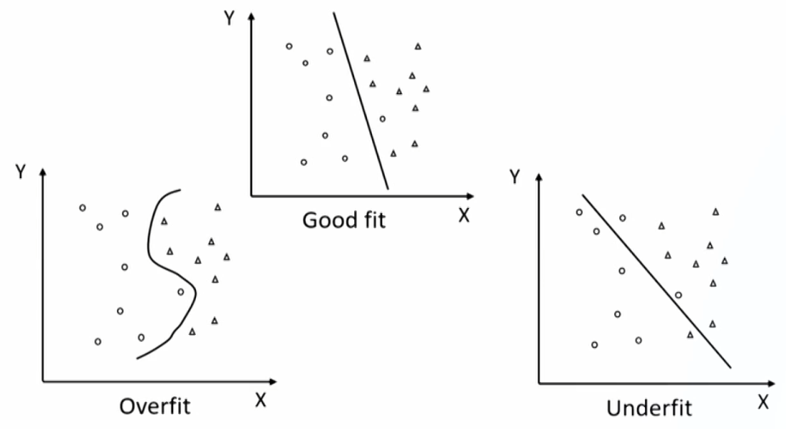
Overfitting and generalization
- Overfitting(过拟合): an ML algorithm fits the training data too well but does not predict well using new data.
- Generalization(泛化): a model with well generalization retains its explanatory power when predicting using new data(out-of-sample).
- A good fit/robust model fits the training (in-sample) data well and generalizes well to out-of-sample data, both within acceptable degrees of error.
Overfitting and errors
- In-sample errors (E_{in}): errors generated by the predictions of the fitted relationship relative to actual target outcomes on the training sample.
- Out-of-sample errors(E_{out}): errors from either the validation or test samples.
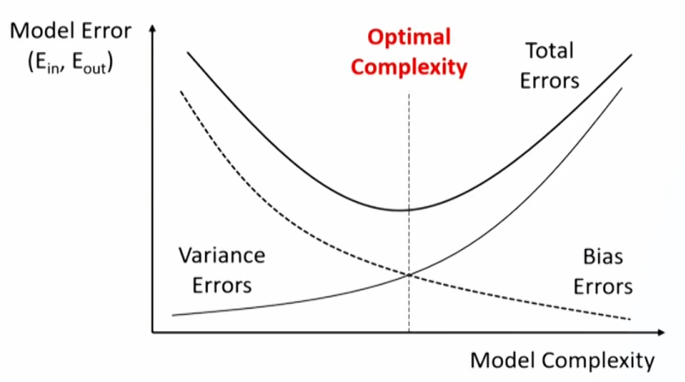
- Total out-of-sample errors can be decomposed into three sources
- Bias error: the degree to which a model fits the training data. 对训练数据学习不足
Algorithms with erroneous assumptions produce high bias,causing underfitting and high in-sample error. - Variance error: how much the model's results change in response to new data from validation and test samples. 对样本外数据泛化能力不足
Unstable models pick up noise and produce high variance,causing overfitting and high out-of-sample error. - Base error: due to randomness in the data. 数据自身随机性
- Bias error: the degree to which a model fits the training data. 对训练数据学习不足
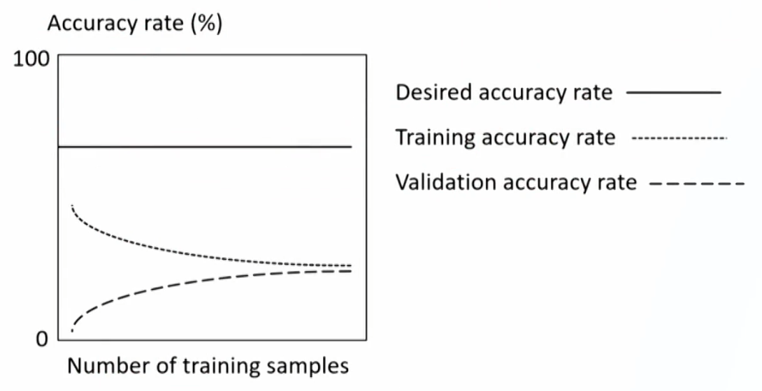
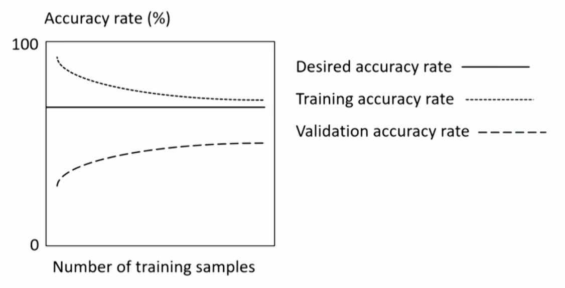
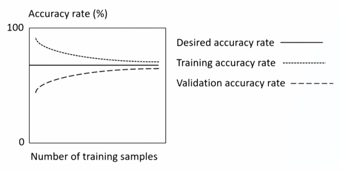
- Learning curve: plots the accuracy rate (1 - error) in the validation or test samples against the amount of data in the training sample.
- It is useful for describing underfitting and overfitting as a function of bias and variance errors.
- Leaning curve for underfitting model: high bias error.
- Leaning curve for overfitting model: high variance error.
- Leaning curve for robust model: good tradeoff of bias and variance error.
- Fitting curve: plots in-sample and out-of-sample error rates(E_{in} and E_{out}) against model complexity.
Prevent overfitting in supervised ML
- Overfitting potential is endemic to the supervised ML due to the presence of noise.Two common principles are used:
- Complexity reduction: limiting the number of features and penalizing algorithms that are too complex.
- Cross-validation: estimating out-of-sample error directly by determining the error in validation samples.
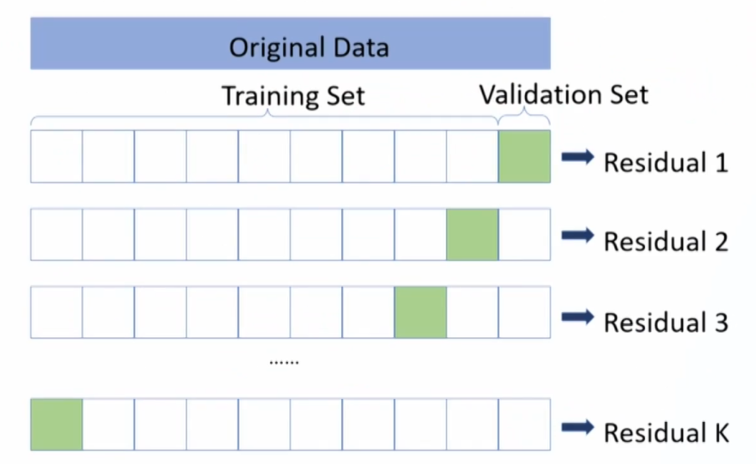
- The problem of holdout samples exists in cross-validation reducing the training set size too much. K-fold cross-validation can mitigate the problem.
- K-fold cross-validation: the data are shuffled randomly and then divided into k equal sub-samples.
- k-1 samples are used as training samples and one sample is used as a validation sample.
- Repeat this process k times.
- The average of the k validation errors is then taken as a reasonable estimate of the model's out-of-sample error.
Supervised Machine Learning Algorithms
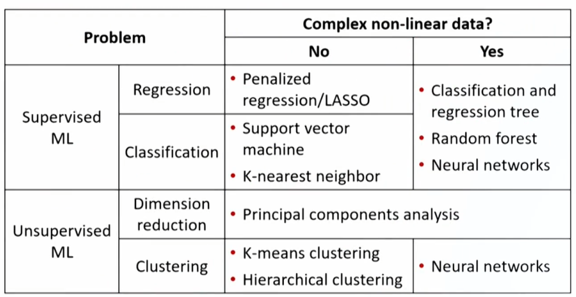
Supervised Machine Learning Algorithms
- Non-Complex non-linear data
- Penalized regression/LASSO
- Support vector machine
- K-nearest neighbor
- Complex non-linear data
- Classification and regression tree
- Random forest
Penalized regression
- In penalized regression, the regression coefficients are chosen to minimize the sum of squared residuals (SSE) plus a penalty term that increases in size with the number of included features.
- So a feature must make a sufficient contribution to model fit to offset the penalty from including it.
- Regularization正则化: tend to selcet parsimonious models which are less subject to overfitting.
- LASSO(least absolute shrinkage and selection operator) is a popular type of penalized regression, and the penalty term has following form:
\text{Penalty term} =\lambda \sum_{\mathrm{k}=1}^{\mathrm{K}}\left|\widehat{\mathrm{b}_{\mathrm{k}}}\right|- \lambda\gt 0, and is a hyperparameter.
- LASSO involves minimizing the sum of the absolute values of the regression coefficients.
Support vector machine
- SVM is a linear classifier that determines the hyperplane(超平面) that optimally separates the observations into two sets of data points.
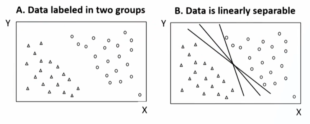
- Linear classifier: a binary classifier that makes its classification decision based on a linear combination of the features of each data point.
- Linear classifier can be represented as straight lines with two dimensions or features, as plane with three dimension of features, and as hyperplane with more than three dimensions features.
- The algorithm of SVM is to maximize the probability of making a correct prediction by determining the boundary that is the furthest away from all the observations.
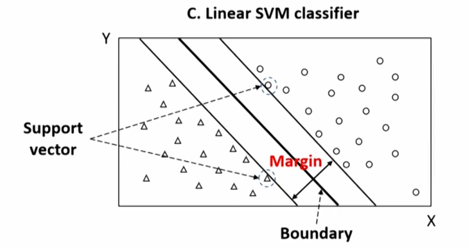
- In real-world, many data sets are not perfectly linearly separable, and two adaption can handle this problem:
- Soft margin classification: adds a penalty to the objective function for observations in the training set that are misclassified, and choose a boundary that optimizes the trade-off between a wider margin and a lower total error penalty.
- Non-linear SVM: introduce more advanced, non-linear separation boundaries.
K-nearest neighbor(KNN,K近邻算法)
- K-nearest neighbor: classify a new observation by finding similarities (nearness) between this new observations and the existing data.
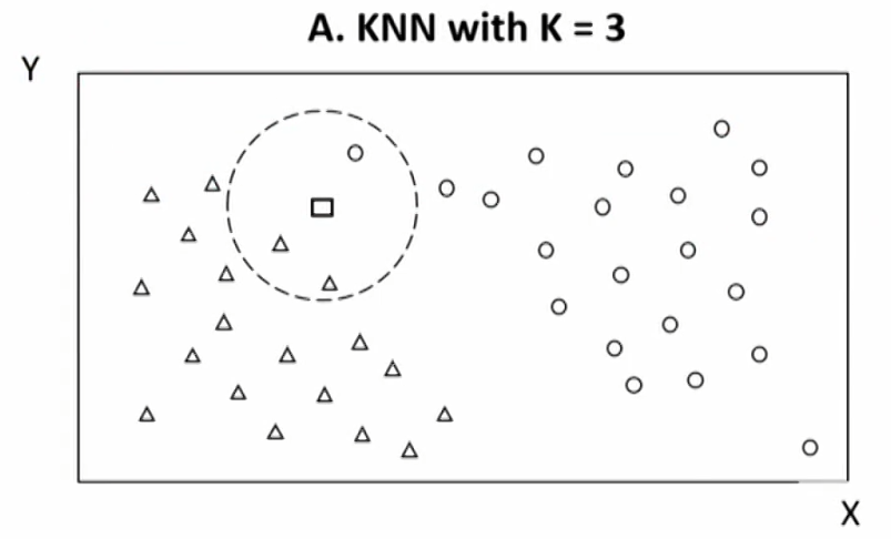
- Decision rule: choose the classification with the largest number of nearest neighbors out of the k being considered
- There are challenges to KNN, two of them are defining "similarity" (nearness) and choosing the value of K.
- An inappropriate measure of "similarity" will generate poorly performing models.
- A too small value for k will result in a high error rate and sensitivity to local outliers, a too large value for k will dilute the concept of nearest neighbors by averaging too many outcomes.
Classification and regression tree
- CART can be applied to predict either a categorical target variable, producing a classification tree, or a continuous outcome, producing a regression tree.
- CART is most commonly used in binary target, and is a combination of an initial root node, decision nodes, and terminal nodes.
- The root node and each decision node represent a single feature and a cutoff value for that feature.
- The same feature can appear several times in a tree in combination with other features.
- Some features may be relevant only if other conditions have been met.
- Example of CART: classify companies by whether or not they increase their dividends
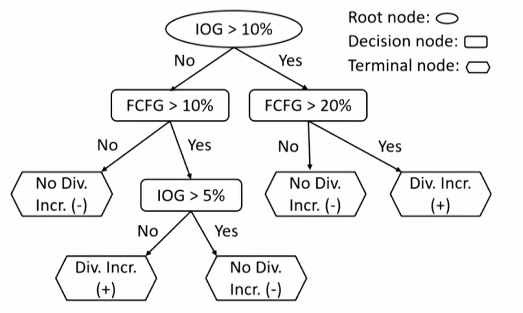
- IOG: investment opportunities growth.
- FCFG: Freecashflowgrowth.
- Feature space.

- The CART algorithm chooses the feature and the cutoff value at root node and each decision node that generates the widest separation of the labeled data to minimize classification error.
- E.g., by a criterion such as mean-squared error.
- At any level of the tree, when the classification error does not diminish much more from another split, the process stops and the node is a terminal node.
- If the objective is classification, then the prediction of at each terminal node will be the category with the majority of data points.
- If the objective is regression, then the prediction at each terminal node is the mean of the labeled values.
- If left unconstrained, CART can potentially perfectly learn the training data. To avoid such overfitting, regularization parameters can be added.
- E.g., the maximum depth of the tree, the minimum population at a node, or the maximum number of decision nodes
- Pruning(模型剪枝): sections of the tree that provide little classifying power are pruned, and can be used afterward to reduce the size of the tree.
Random forest
- Ensemble learning(集成学习) combines the prediction from a collection of models, and can be divided into two main categories:
- Voting classifier: aggregation of heterogeneous learners (i.e different types of algorithms).
Majority-vote classifier(少数服从多数) - Bootstrap aggregating(or bagging): aggregation of homogenous learners (i.e., same algorithm using different training data).
Random sampling with replacement
- Voting classifier: aggregation of heterogeneous learners (i.e different types of algorithms).
- A random forest classifier is a collection of a large number of CART trained via a bagging method.
- To derive more diversity in the trees, one can randomly reduce the number of features available during training.
- If each observation has n features, one can randomly select a subset of m features (where m < n).
- For any new observation, we let all the classifier trees undertake classification by majority vote.
Unsupervised Machine Learning Algorithms
Unsupervised Machine Learning Algorithms
- Dimension reduction
- Principal Components Analysis
- Clustering
- K-means Clustering: with fixed number(k) of categories.
- Hierarchical Clustering: without fixed number of categories.
Principal components analysis
- PCA is used to summarize or reduce highly correlated features of data into a few main, uncorrelated composite variables.
- Composite variable(复合变量): a variable that combines two or more variables that are strongly related to each other.
- PCA involves transforming the covariance matrix of the features, and involves two key concepts:
- Eigenvectors(特征向量): new, mutually uncorrelated composite variables that are linear combinations of the original features.
- Eigenvalues(特征值): the proportion of total variance in the initial data that is explained by each eigenvector.
- To find the principal components (PCs), we follow two rules
- Minimize the sum of the projection errors for all data points.
Projection error: the vertical distance between the data point and PC. - Maximize the sum of the spread between all the data.
Spread: the distance between each data point in the direction that is parallel to PC.
- Minimize the sum of the projection errors for all data points.
- PCA algorithm orders the eigenvectors from highest to lowest according to their eigenvalues.
- Step 1: standardize the data so that the mean of each series is 0 and the standard deviation is 1.
- Step 2: find the first PC according to the rules.
- Step 3: find the second PC which is at right angles to the first PC thus is uncorrelated with the first PC.
- Step 4: go on until the most part of total variance in the data is explained by the PCs.
- Scree plots show the proportion of total variance in the data explained by each principal component.
K-means clustering
- K-means clustering repeatedly partitions observations into a fixed number (k) of non-overlapping clusters.
- Each cluster is characterized by its centroid 中心点.
- Each observation is assigned by the algorithm to the cluster with the centroid to which that observation is closest.
- Steps of k-means algorithms:
- Step 1: determine the position of the k initial random centroids.
- Step 2: assigns each observation to its closest centroid which defines a cluster.
- Step 3: calculates the new (k) centroids for each cluster.
- Step 4: reassigns the observations to the new centroids, and redefine the clusters.
- Step 5: repeat the process of recalculating the new centroids,reassigning the observations and redefining the new clusters.
- Step 6: stop the algorithm when no observation is reassigned to a new cluster, and the final k clusters are revealed.
Hierarchical clustering
- Hierarchical clustering is an iterative procedure used to build a hierarchy of clusters很多层级的类别, creating intermediate rounds of clusters of increasing(agglomerative, 合成) or decreasing(divisive, 分裂) size until a final clustering is reached.
- Agglomerative clustering(or bottom-up):合成聚类
- Divisive clustering(or top-down):分裂聚类
- Agglomerative clustering begins with each observation being treated as its own cluster. Then the algorithm finds the two closest (most similar) clusters and combines them into one new larger cluster. This process is repeated iteratively until all observations are clumped into a single cluster.
- Is well suited for identifying small clusters.
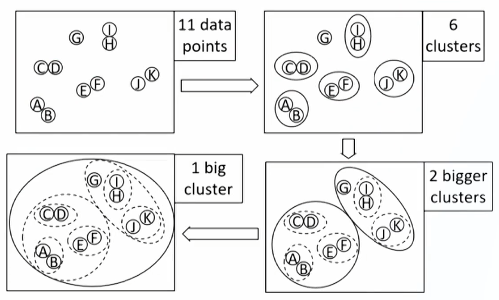
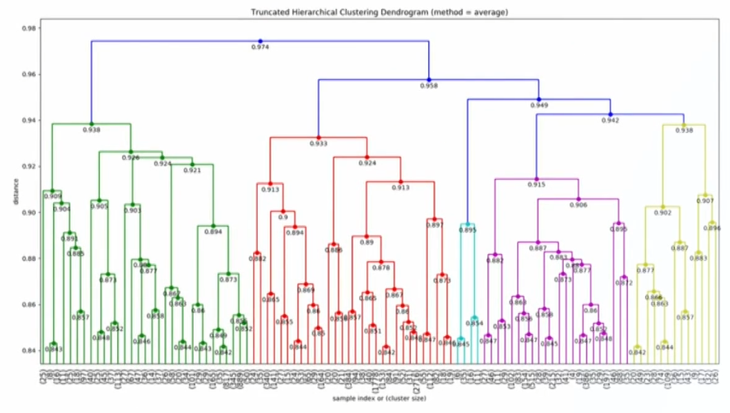
- Dendrogram: tree diagram for visualizing a hierarchical cluster
- Is well suited for identifying small clusters.
- Divisive clustering begins with all the observations belonging to a single cluster. The observations are then divided into two clusters based on some measure of distance (similarity). The algorithm then progressively partitions the intermediate clusters into smaller clusters until each cluster contains only 1 observation.
- Is better suited for identifying large clusters.