VaR and other risk measures
Introduction and Overview
Parametric Approach
- Value at Risk(VaR): The minimum loss that would be expected a certain percentage of the time over a certain period of time given the assumed market conditions.
- Example: the 5% VaR of a portfolio is £2.2 million over a one-day period.
- Interpretation: 5% probability of losses of at least $2.2 million(minimum loss) in one day or 95% probability of losses of at most $2.2 million(maximum loss) in one day.
- Parametric approach requires to specify the statistical distribution from which our data observations are drawn.
- Parametric approaches can be thought of as fitting curves through the data and then reading off the VaR from the fitted curve.
- Normal VaR
- Assume P/L(or arithmetic return) is normally distributed.
\begin{aligned} & \operatorname{VaR_\%}(\alpha)=-\left(\mu_r-z_\alpha \times \sigma_r\right) \\ & \operatorname{VaR_\$}(\alpha)=-\left(\mu_r-z_\alpha \times \sigma_r\right) \times P_{t-1} \\ & \operatorname{VaR_\$}(\alpha)=-\left(\mu_{P / L}-z_\alpha \times \sigma_{P / L}\right)\end{aligned}
\alpha : significance level;
1-\alpha : confidence level。
\mathrm{z}_\alpha : the standard normal variate corresponding to \alpha。
\mu_{P / L} : the mean of P / L。
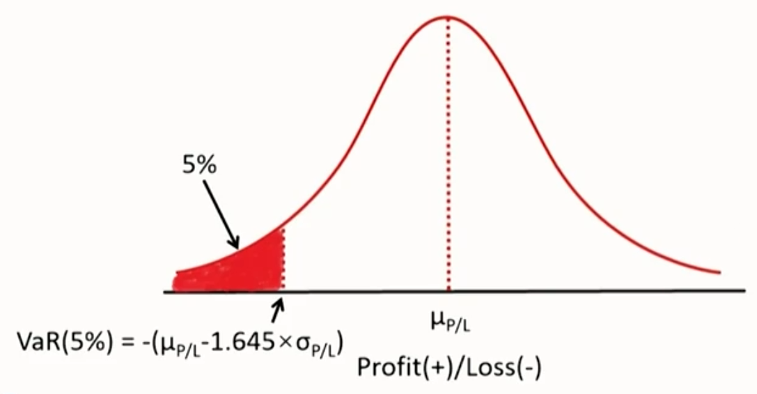
\sigma_{P / L}: the standard deviation of P / L - Graphical representation of normal VaR(5%):
- Assume P/L(or arithmetic return) is normally distributed.
- Lognormal VaR
- Assume that geometric returns are normally distributed
Since the VaR is a loss, or the difference between P (which is random) and Pt-1 (which can be taken as given), then the VaR itself has the same distribution as Pt
Normally distributed geometric returns imply that the VaR is lognormally distributed. - Formula to calculate the lognormal VaR:
\begin{aligned} & \operatorname{VaR_\%}(\alpha)=\left(1-e^{\mu_R-z_\alpha \times \sigma_R}\right) \\ & \operatorname{VaR_\$}(\alpha)=\left(1-e^{\mu_R-z_\alpha \times \sigma_R}\right) \times P_{t-1}\end{aligned}
\alpha : significance level
1-\alpha : confidence level。
z_\alpha : the standard normal variate corresponding to \alpha。
\mu_{\mathrm{R}} : the mean of geometric returns。
\sigma_R : the standard deviation of geometric returns
- Assume that geometric returns are normally distributed
- 如果时间跨度不同,用均值除以天数,用标准差除以天数的平方根
Expected shortfall(ES)
- Disadvantages of VaR
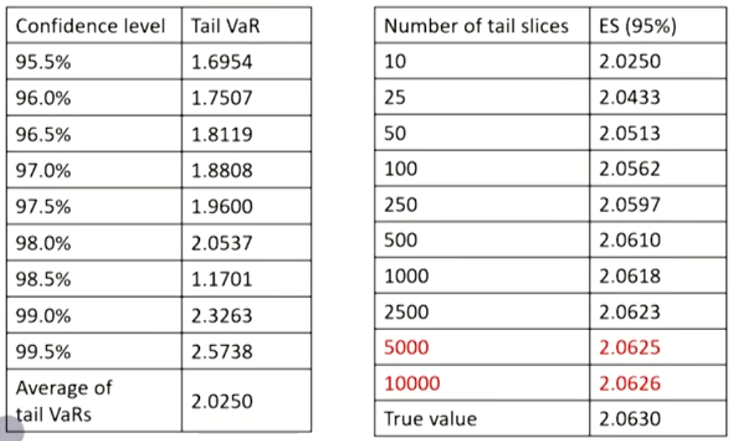
- VaR only provides the minimum loss for a given percentage (significance level, a), but it does not tell the magnitude of the actual loss. While the ES is the probability-weighted average of tail losses, which can be estimated as an average of "tail VaRs"在大于区间内平均切片,对应值的平均值就是ES
- VaR is not subadditive, so VaR is not a coherent risk measure. While ES is a coherent risk measure.
- As the number of slices increases,ES converges to true value.切的多,ES增加
Standard errors of quantile (VaR) estimators
- Standard errors, or (generally better) confidence intervals can be used to evaluate precision of estimators of risk measures.Formula to calculate the standard errors(SE):
S E(q)=\left[\frac{p \times(1-p)}{n {f(q)}^2}\right]^{1/2}- p: the proportion for the quantile。
- {f(q)} : the corresponding probability density function
- Two conclusions derived from the SE formula:
- SE falls as the sample size n rises.
- SE rises as the probabilities is more extreme.
- Confidence intervals around the quantile estimators:
\left[q-Z_{\frac{\alpha}{2}} \times S E(q), q+Z_{\frac{\alpha}{2}} \times S E(q)\right]
Quantile-Quantile(QQ) plots
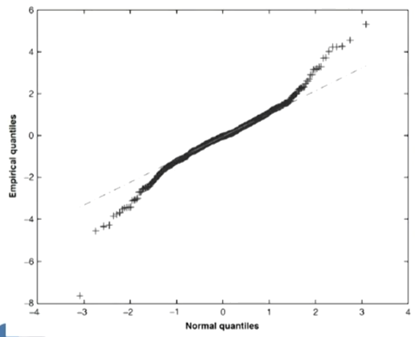
- QQ plot is a plot of the quantiles of the empirical distribution against those of some specified (or reference) distribution,and can be used to identify the distribution of our data by its shape
- A linear QQ plot tells the specified distribution fits the data.
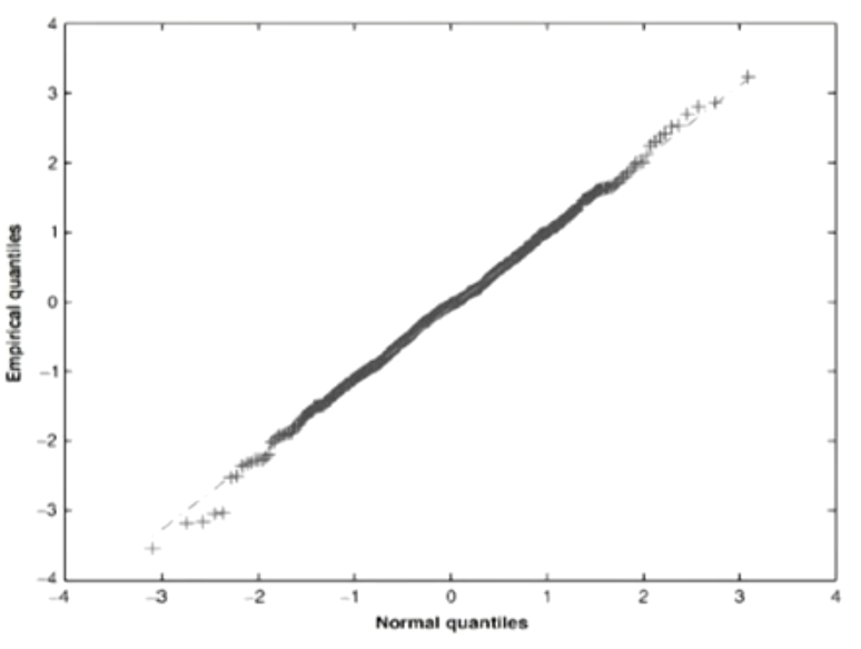
- Departures of the QQ plot from linearity in the tails can tell that the tails of empirical distribution are fatter or thinner than the tails of the reference distribution.
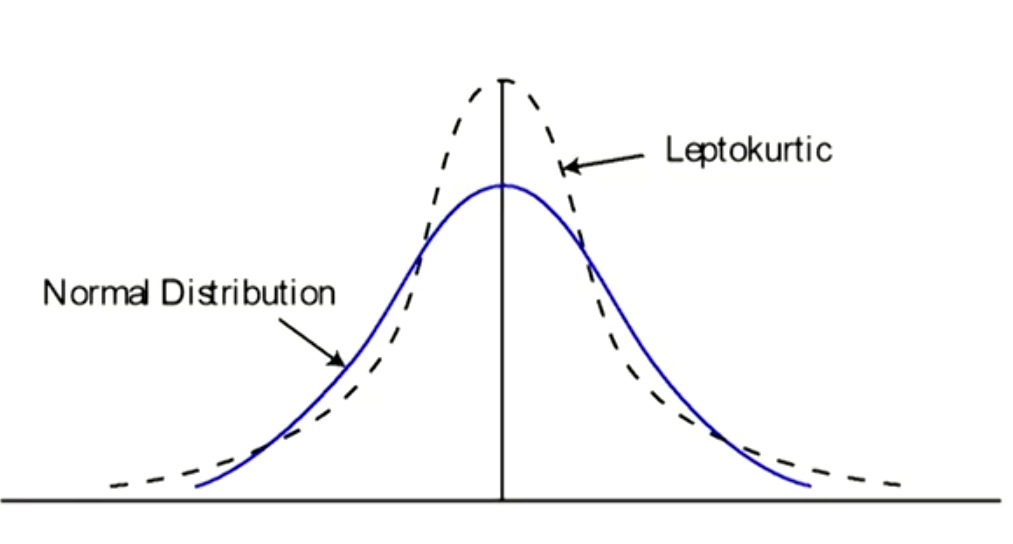
- If the empirical distribution has heavier tails(leptokurtosis, 峰度大于3) than the reference distribution, the QQ plot will have steeper slopes at its tails.
Non-parametric Approaches
Historical simulation (HS) approach
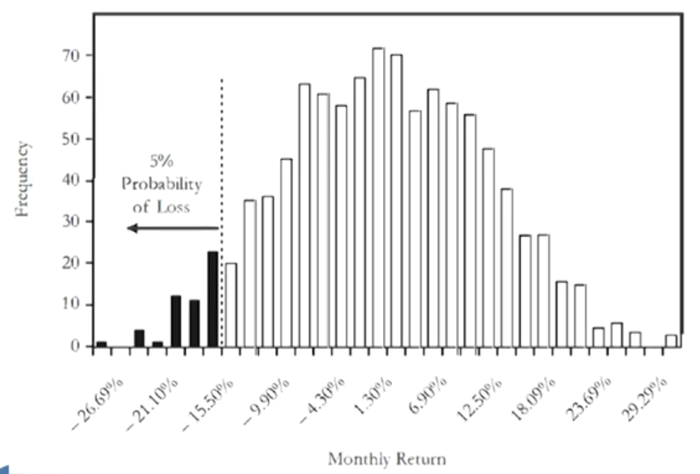
- The HS approach estimates VaR by means of ordered loss observations
- HS specifies an equal weight for observations that occurred after the cutoff date but a zero weight for observations that occurred before the cutoff date.
- In practice, HS VaR estimates can be obtained from a cumulative histogram, or empirical cumulative frequency function.
Bootstrap historical simulation
- Bootstrap historical simulation is one simple but powerful method to improve the estimation precision of VaR and ES over basic historical simulation用Bootstrap能提升Var和ES的精确度
- A bootstrap procedure involves resampling from our existing data set with replacement放回.
- Steps to apply the bootstrap:
- create a large number of new samples at random from our original sample with replacement.
- each new 'resampled'sample gives us a new VaR or ESestimate.
- take the 'best'estimate to be the mean of these resample-based estimates.每次抽样计算一次,平均值作为最终结果
Non-parametric density estimation
- Basic historical simulation has a practical drawback that VaRs can only be estimated at discrete confidence intervals determined by the size of our data set.
- Example: the VaR at the 95.1% confidence level is not available wit basic historical simulation if there is only 100 P/L observations.
- Non-parametric density estimation offers a potential solution to this problem.
- Treat our data as if they were drawings from some unspecified or unknown empirical distribution function.
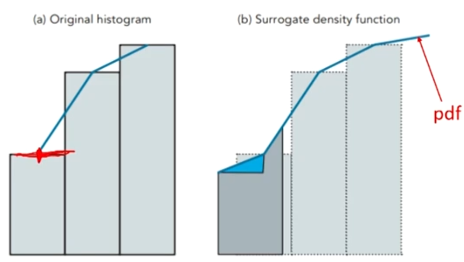
Draw lines through mid-points on the edges of the 'bars'of a histogram.
Treat the areas under these lines as a surrogate(近似代替的) probability density function.
Proceed to estimate VaRs for arbitrary confidence levels.
- Treat our data as if they were drawings from some unspecified or unknown empirical distribution function.
Traditional historical simulation
- In the traditional historical simulation, the weight of the past observation is either 1/n (in sample period) or 0 (beyond sample period) if the sample size is n.
- This weighting structure has a number of problems:
- It is hard to justify giving each observation the same weight,regardless of age, market volatility, or anything else.
- Equal-weight structure makes risk estimates unresponsive(反应迟滞的)to major events.
- Periods of high and low volatility tend to be clustered.
- An observation will have a weight that suddenly goes to zero when it reaches age n.
- Creates the potential for "ghost effects(鬼影效应)": have a VaR that is unduly(异常地)hig because of a small cluster of high loss observations, and the measured VaR will continue to be high until n days have passed and the observation has fallen out of the sample period.
Age-weighted historical simulation (BRW)
- It gives relative weights of our observations by age (discount older observations in favor of newer ones), as suggested by Boudoukh, Richardson and Whitelaw(BRW: 1998).

w_{(1)}:the weight given to an observation1day old:
\begin{gathered} w_{(1)}+\lambda w_{(1)}+\lambda^2w_{(1)}+\cdots+\lambda^{n-1} w_{(1)}=1\\ w_{(1)}=\frac{1-\lambda}{1-\lambda^n} \end{gathered}
w_{(i)}: the weight given to an observation i day old:
w_{(i)}=\frac{\lambda^{i-1}(1-\lambda)}{1-\lambda^n} - The age-weighted approach has four major attractions:
- It provides a nice generalization of traditional historical simulation (HS), because traditional HS can be regarded as a special case with zero decay, or λ = 1.传统历史模拟法是特例
- A suitable choice of λ can make the VaR(or ES) estimates more responsive to large loss observations.更关注近期数据
A large loss event will be given a higher weight than under traditional HS, and the resulting next-day VaR would be higher than it would otherwise have been. - It helps to reduce distortions caused by events that are unlikely to recur, and helps to reduce or eliminate ghost effects.减少鬼影效应
- It gives us the option of letting our sample size grow over time.可以包括很多数据
Volatility-weighted historical simulation (HW)
- This approach weights data by volatility, updates return information to take account of recent changes in volatility,suggested by Hull and White (HW; 1998)
r_{t, i}^*=\left(\frac{\sigma_{T, i}}{\sigma_{t, i}}\right) \times r_{t, i}
r_{t, i}: actual return for asset \mathrm{i} on day \mathrm{t}。
\sigma_{t, i}: volatility forecast for asset \mathrm{i} on day \mathrm{t}。
\sigma_{T, i}: current forecast of volatility for asset \mathrm{i}。 - Estimate VaR or ES with the adjusted return data set, instead of the original return data set.
- Actual returns in any period t are therefore increased (or decreased), depending on whether the current forecast of volatility is greater (or less) than the estimated volatility for period t.
- Advantages of volatility-weighted historical simulation:
- It directly takes account of volatility changes and produces risk estimates that incorporate information of current volatility estimates.考虑了波动率预测值的影响
- It can obtain risk estimates that can exceed the maximum loss in historical data set.收益率可以超过历史最大值
- Empirical evidence indicates that this approach produces superior VaR estimates.可以带来更好的VaR估计
Correlation-weighted historical simulation
- This approach adjusts historical returns to reflect changes between historical and current correlations.类似波动率加权,不过基于历史波动率
- It is achieved by multiplying historic returns by revised correlation matrix(equivalently variance-covariance matrix) to yield updated correlation-adjusted returns.
- It is more involved and richer than volatility-weighting because it allows for updated variances (volatilities) as well as covariances(correlations).
Filtered historical simulation
- The most comprehensive and most complicated approach.最负责
- This approach is a form of semi-parametric一半参数一半非参 bootstrap which aims to combine the benefits of HS with the explanatory power and flexibility of conditional volatility models such as GARCH to capture varying volatility and volatility clustering.
- It preserves the non-parametric nature of HS by bootstrapping returns, using parametric volatility model
- Empirical evidence supports the predictive ability效果好.
Advantages of non-parametric approaches
- Intuitive and conceptually simple.
- Use data that are (often) readily available.历史数据容易获得
- Provide results that are easy to report and communicate.
- Easy to implement on a spreadsheet.
- Easy to produce confidence intervals.
- Capable of considerable refinement and potential improvement.容易提升
- Combine them with parametric 'add-ons' to make them semi-parametric.
- Can accommodate any non-normal features that can cause problems for parametric approaches due to dependence on parametric assumptions about P/L.适用性强
- Can theoretically accommodate any type of position,including derivatives positions.
- Free of the operational problems that parametric methods are subject to when applied to high-dimensional problems
- No need for covariance matrices, no curses of dimensionality, etc.不依赖协方差矩阵
Disadvantages of non-parametric approaches
- The results are very dependent on the historical data set.历史无法代表未来
- If the sample period was unusually quiet (volatile), the VaR or ES estimates will be too low (high) for the risks we are actually facing
- Difficult to handle shifts that take place during our sample period, and sometimes slow to reflect major events.对重大事件反应慢
- Extreme losses in sample period, even though it is not expected to recur, can dominate risk estimates.历史极端情况不一定适合现在
- Subject to the phenomenon of ghost or shadow effects.有鬼影效应
- Make no allowance for plausible events that might occur, but did not actually occur in our sample period.没有考虑未来时间
- The VaR and ES estimates are constrained by the largest loss in our historical data set (greater or lesser extent).
Parametric Approaches
Generalized extreme-value(GEV)广义极值分布
- Extreme value
- Extreme events are unlikely to occur, so the challenge is that few extreme observations make estimation difficult.
- The result of efforts is extreme-value theory (EVT), a branch of applied statistics:
EVT is quite different from the more familiar "central tendency" statistics, which are governed by central limit theorems, but central limit theorems do not apply to extremes.
- Generalized extreme-value theory
- As sample size n gets large, the distribution of extremes converges to the generalized extreme-value (GEV) distribution.样本极端值的分布
\begin{aligned} & H_{\xi, \mu, \sigma}=\exp \left[-\left(1+\xi \frac{X-\mu}{\sigma}\right)^{-\frac{1}{\xi}}\right], \text { if } \xi \neq0; \\ & H_{\xi, \mu, \sigma}=\exp \left[-\exp \left(\frac{X-\mu}{\sigma}\right)\right], \text { if } \xi=0.\end{aligned}
\mu : the location parameter of the distribution。
\sigma : the scale parameter of the limiting distribution。
\xi: the tail index, gives an indication of the shape (or heaviness) of the tail of the limiting distribution。 - If \xi\gt0, the GEV becomes the Frechet distribution. In this case tail is heavy, and particular useful for financial returns. The tail is similar with Levy, t and Pareto distribution.
- If \xi = 0, the GEV becomes the Gumbel distribution. In this case, tail is light. Tail is similar with normal and lognormal distribution.
- If \xi\lt0, the GEV becomes the Weibull distribution. In this case, tail is lighter, few empirical financial return are so light-tailed.
- If we are confident that we can identify the parent loss distribution, we can choose the EV distribution.
For example, if the original distribution is a t, then we would choose the Frechet distribution. - We can test the significance of tail index, and we may choose Gumbel if the tail index is insignificant and Frechet otherwise
- Given the dangers of model risk and bearing in mind that the estimated risk measure increases with the tail index, a safer option is always to choose the Frechet.
- As sample size n gets large, the distribution of extremes converges to the generalized extreme-value (GEV) distribution.样本极端值的分布
Peaks-over-threshold(POT)
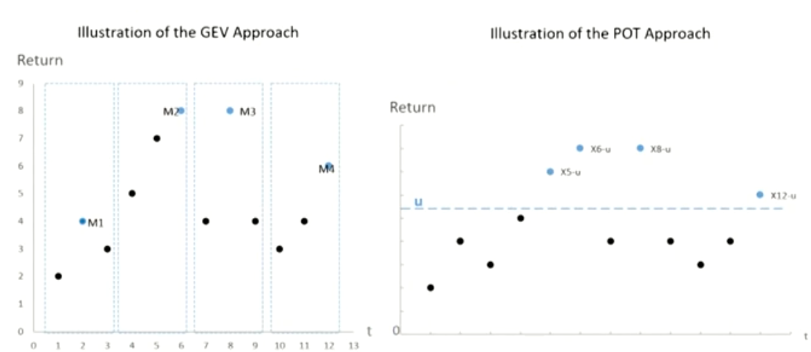
- Peaks-over-threshold (POT) deals with the application of EVT to the distribution of excess losses over a high threshold.超过阈值的样本的分布
- POT approach models exceedances over a high threshold,while GEV models maxima or minima of a large sample.
- Probability
F_u(x)=P\{X-u \leq x \mid X>u\}=\frac{{F(x+u)}-{F(u)}}{1-{F(u)}}- The distribution of X itself can be any of the commonly used distributions: normal, lognormal, t.
- Gnedenko-Pickands-Balkema-deHaan (GPBdH) theorem states that the distribution \mathrm{F}_{\mathrm{u}}(\mathrm{x}) converges to a generalized Pareto(GP) distribution阈值越大,越趋向于广义帕累托分布
\begin{aligned} &1-\left(1+\frac{\xi x}{\beta}\right)^{-\frac{1}{\xi}}, \text { if } \xi \neq0\\ &1-\exp \left(-\frac{x}{\beta}\right), \xi=0\end{aligned}
This distribution has only two parameters: a positive scale parameter \beta, and a shape or tail index parameter \xi
- POT and GP distribution
- To apply the GP distribution, a reasonable threshold u, which determines the number of observations,Nu, in excess of the threshold value.
- Choosing u involves a trade-off: we want a threshold u to be sufficiently high for the GPBdH theorem to apply reasonably closely. However, if u is too high, we won't have enough excess-threshold observations on which to make reliable estimation.
VaR and ES using POT
\begin{aligned} & V a R=u+\frac{\beta}{\xi}\left\{\left[\frac{n}{N_u}(1-\text { confidence level })\right]^{-\xi}-1\right\} \\ & E S=\frac{V a R}{1-\xi}+\frac{\beta-\xi u}{1-\xi}\end{aligned}- \mathrm{u} is reasonable threshold in percentage term
- \mathrm{N}_{\mathrm{u}} is number of the observations exceeding threshold
- \mathrm{n} is the total observations
GEV vs. POT
- POT approach models exceedances over a high threshold, while GEV models maxima or minima of a large sample多变量极值的分布
- GEV has three parameters (\xi, \mu, \sigma) to estimate,while POT only has two parameters (\beta, \xi)。
- POT needs to choose a threshold
Multivariate EVT(MEVT)
- MEVT can be used to model the tails of multivariate distributions in a theoretically appropriate way. Modeling of multivariate extremes requires us to make use of copulas,which enables us to use as many dimensions as we like.
- Curse of dimensionality: As the dimensionality rises,multivariate EV events rapidly become much rarer.变量太多,估计的参数太多,估计不过来
- The occurrence of multivariate extreme events depends on their joint distribution, and extreme events cannot be assumed to be independent.极端事件之间一般不独立
- More independent variables in multivariate distributions allows a less number of extreme observations to be generated for modeling tail distributions.更多的独立变量导致极端值越少
Backtesting VaR
Definitions
- Backtesting: a formal statistical framework that consists of verifying that actual losses are in line with projected losses.
- This involves systematically comparing the history of VaR forecasts with their associated portfolio returns.
- If the VaR forecasts are not well calibrated, the models should be reexamined for faulty assumptions, wrong parameters, or inaccurate modeling.
- Exception: observations falling outside VaR.
- Too many exceptions means the model underestimates risk.
Problem: too little capital may be allocated to risk-taking units; penalties also may be imposed by the regulator. - Too few exceptions means the model overestimates risk.
Excess, or inefficient, allocation of capital across units.
- Too many exceptions means the model underestimates risk.
- Failure rate: the proportion of times VaR is exceeded in a given sample.
- Failure rate = N/T; N: the number of exceptions.
- Ideally, the failure rate should give an unbiased measure of p, or should converge to p as the sample size increases.
p: the percentage of left-tail level for VaR figure.
Difficulties in backtesting VaR models
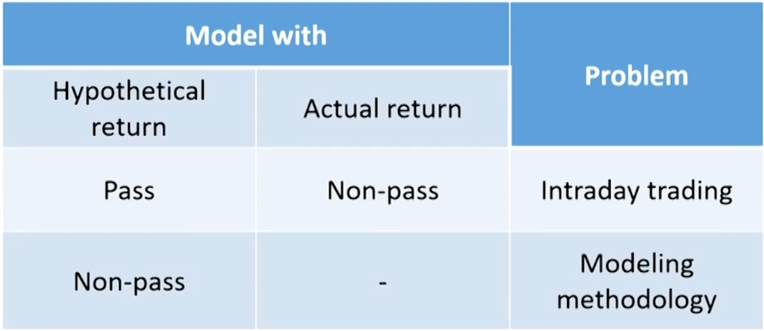
- Risk manager should track both the actual portfolio return and the hypothetical return.
- Actual return: corresponds to the actual P&L, taking into account intraday trades and other profit items such as fees,commissions, spreads, and net interest income.
- Hypothetical return: obtained from frozen portfolios (freezing the starting positions) applied to the actual returns on all securities, measured from close to close.假想一个组合,算每日收益率
- Cleaned return: the actual return minus all non-mark-to-market items, such as fees, commissions, and net interest income
- Under the latest update to the market-risk amendment,supervisors will have the choice to use either hypothetical or cleaned returns.
- Validation
- If the model passes backtesting with hypothetical but not actual returns, then the problem lies with intraday trading
- If the model does not pass backtesting with hypothetical returns, then the modeling methodology should be reexamined.
Model verification
- A test can be applied to verify the model when T is large.
- H0: the model is correctly calibrated.模型有用
z=\frac{x-p T}{\sqrt{p(1-p) T}} \sim N(0,1)
x: the number of exceptions.例外的个数
x/T: the failure rate. - According to the test confidence level, the cutoff value(critical value) can be obtained, such as ±1.96 for two tailed 95% test confidence level.
- H0: the model is correctly calibrated.模型有用
- Unconditional coverage model
- This model ignores conditioning, or time variation in the data.
The exceptions should be evenly spread over time. - Kupiec(1995) develops a 95% confidence region test, defined by the tail points of the log-likelihood ratio:
L R_{u c}=-2\ln\left[(1-p)^{T-X} p^X\right]+2\ln\left[\left(1-\frac{X}{T}\right)^{T-X}\left(\frac{X}{T}\right)^X\right]
H_0 : the model is correctly calibrated模型有用
L R_{u c} is asymptotically(i.e., when \mathrm{T} is large) distributed chis-quare with one degree of freedom
Reject the H_0 if the L R_{u c}\gt 3.84。 - Non-rejection regions at 95% test confidence:
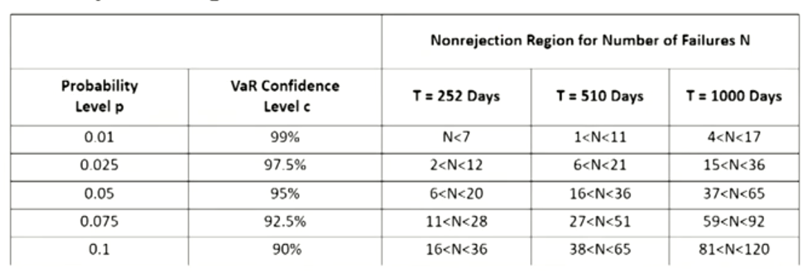
E.g , with T = 510 days and p = 0.01, the Ho will not be reject as long as N is within the [1 < N < 11] confidence interval.
- Conclusion 1: the interval expressed as a proportion N/T shrinks as the sample size increases.
With more data, the model should be able to be rejected more easily if it is false. - Conclusion 2: For small values of the VaR parameter p, it becomes increasingly difficult to confirm deviations.
There is no way to tell N is abnormally small and the model systematically overestimates risk.
- This model ignores conditioning, or time variation in the data.
- Conditional coverage model
- Conditional coverage means the observed exceptions could cluster or bunch扎堆 closely in time, which invalidate the unconditional coverage model.
- Then for conditional coverage, the overall test statisti is
L R_{c c}=L R_{u c}+L R_{i n d}
If L R_{c c}\gt 5.991, H_0 can be rejected模型无用
If L R_{\text {ind }}\gt 3.841, independence alone can be rejected是Conditional coverage model
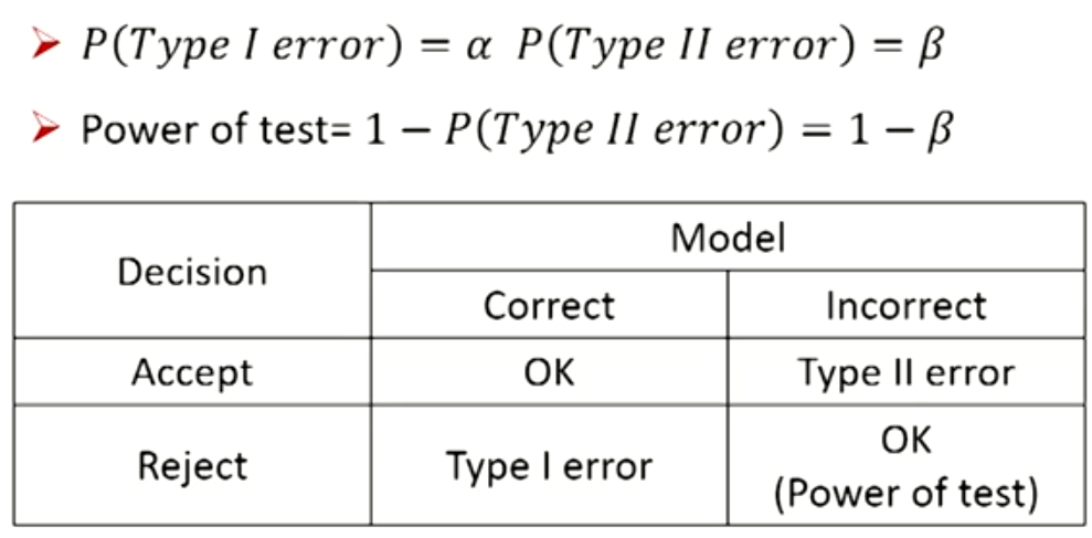
Type I and Type Il error
- A Type I error is committed when a correctly specified model is rejected.
- A Type II error is committed when an incorrectly specified model is accepted.
- A backtest is considered statistically powerful if it minimizes both the probability of committing a Type I error and the probability of committing a Type ll error.
- The probabilities of committing Type I error and Type II error decrease when the sample size increases.
The Basel rules for backtesting
- Backtesting is central to the Basel Committee's ground- breaking decision(突破性决策) to allow internal VaR(99%) models for capital requirements.
- It is unlikely the Basel Committee would have done so without the discipline of a rigorous backtesting mechanism.
- Otherwise, banks may tend to understate their risk.
- The Basel Committee has decided that up to four exceptions are acceptable,otherwise incurs a progressive penalty(渐进 式惩罚)of increasing the multiplicative factor k from 3 to 4.
- The Basel penalty zones:
- k: the multiplicative factor
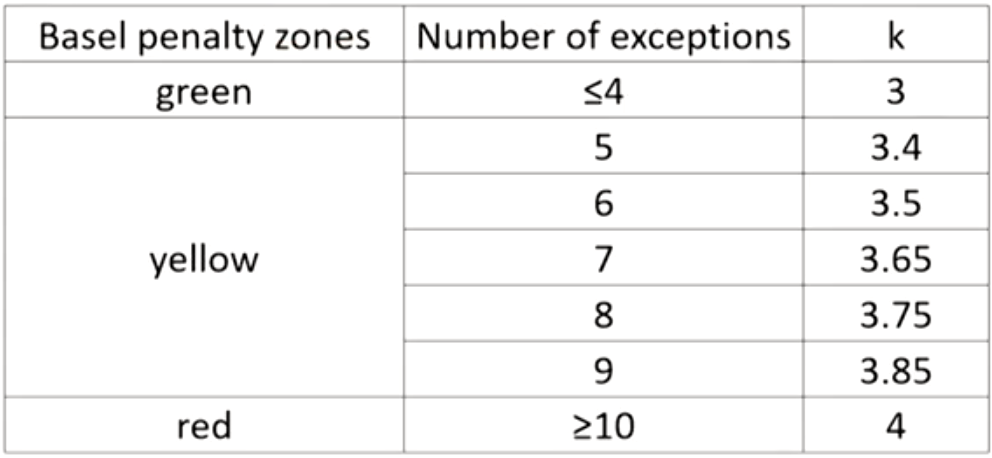
- Within the "red" zone generates an automatic penalty.
- Within the "yellow" zone, the penalty is up to the supervisor,depending on the reason for the exception. The Basel Committee uses the following categories:
Basic integrity of the model: the positions were reported incorrectly or an error in the program code. The penalty should apply".
Model accuracy could be improved: the model does not measure risk with enough precision. The penalty "should apply".
Intraday trading: positions changed during the day. The penalty "should be considered."
Bad luck: markets were particularly volatile or correlations changed. Gives no guidance except that these exceptions should "be expected to occur at least some of the time."
- k: the multiplicative factor
VaR Mapping
Why mapping
1、 The portfolio generally involves a very large number of positions, including bonds, stocks, currencies, commodities,and their derivatives.
- It would be too complex and time-consuming to model all positions individually as risk factors.
- Mapping provides a shortcut, the positions can be simplified to a smaller number of positions on a set of elementary(基本的),or primitive (原始的),risk factors.
- Mapping is also required as a solution to data problems in many common situations.
- Risk manager would have to replace these positions by exposures on similar risk factors already in the system.
- Stale prices are not synchronously(同步地) created, daily correlations across markets are too low, which will affect the measurement of portfolio risk.
Definition of VaR mapping
- A process by which the current values of the portfolio positions are replaced by exposures on the risk factors.把组合的VaR映射成底层因子的VaR
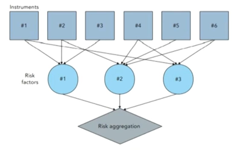
- The mapping process
- Step 1: marking all positions to market in current dollars or whatever reference currency is used.
- Step 2: the market value for each instrument then is allocated to the risk factors.
- Step 3: positions are summed for each risk factor.
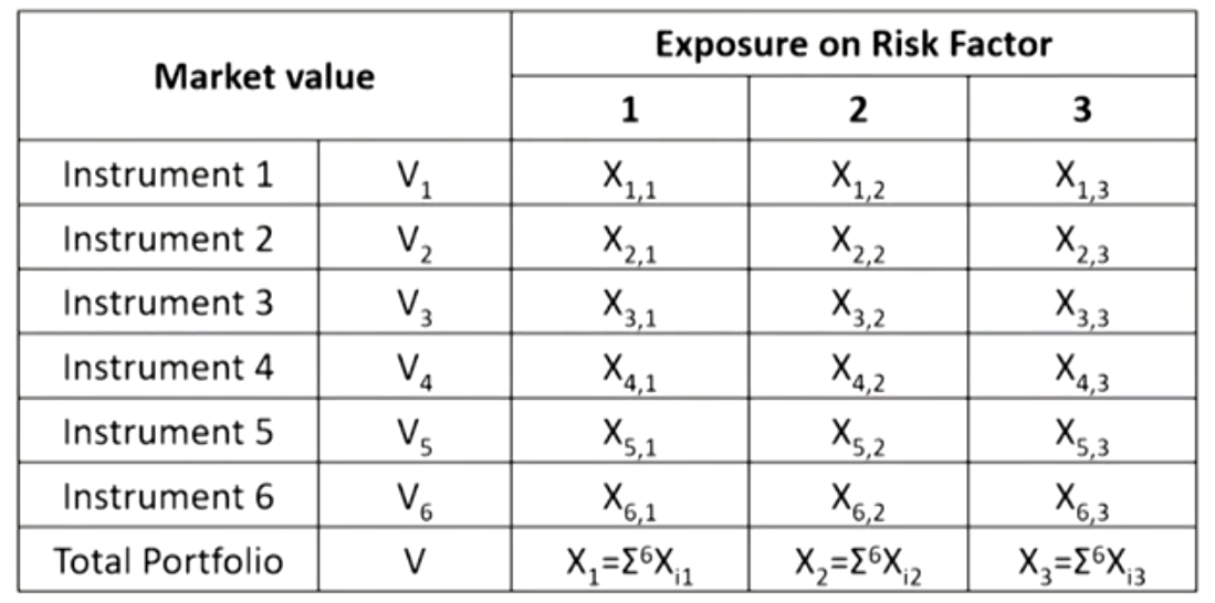
- Mapping can be of two kinds:
- The first provides an exact allocation of exposures on the risk factors.The price is an exact function of the risk factors(such as derivatives).
- The second exposures may have to be estimated.This occurs when a stock is replaced by a position in the stock index.
General and specific risk
- The choice of the set of general (primitive) risk factors should reflect the tradeoff between better quality of the approximation and faster processing.
- Too many risk factors would be unnecessary, slow, and wasteful.
- Too few risk factors could create blind spots in the risk measurement system.
- The choice of primitive risk factors also influences the size of specific risks.
- Specific risk: risk due to issuer-specific price movements,after accounting for general market factors.
- The definition of specific risk depends on that of general market risk.
- A greater number of general risk factors should create less residual risk.系统性风险因子越多,非系统性风险风险越少
Methods of mapping fixed income portfolios
- Zero-coupon bonds can be selected to be the standard instruments to map the fixed-income portfolio.
- The risk percentage or VaR percentage for zero-coupon bonds can for different maturities can be calculated as follows:
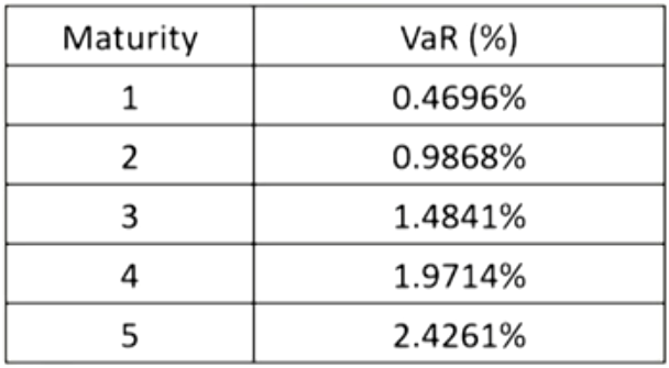
- The risk percentage or VaR percentage for zero-coupon bonds can for different maturities can be calculated as follows:
- Principal mapping: one risk factor is chosen that corresponds to the average portfolio maturity.用平均期限对应的零息债券的VaR
- It overstates the true risk and is the less precise method.忽略票息导致偏高
- Duration mapping: one risk factor is chosen that corresponds to the portfolio duration.用平均久期相同的零息债券的VaR
- It is the less precise method.
- Cash-flow mapping: the portfolio cash flows are grouped into maturity buckets, mapping to many risk factors.每笔现金流视为零息债券分别求VaR
- It is the most precise method
- Undiversified VaR and Diversified VaR
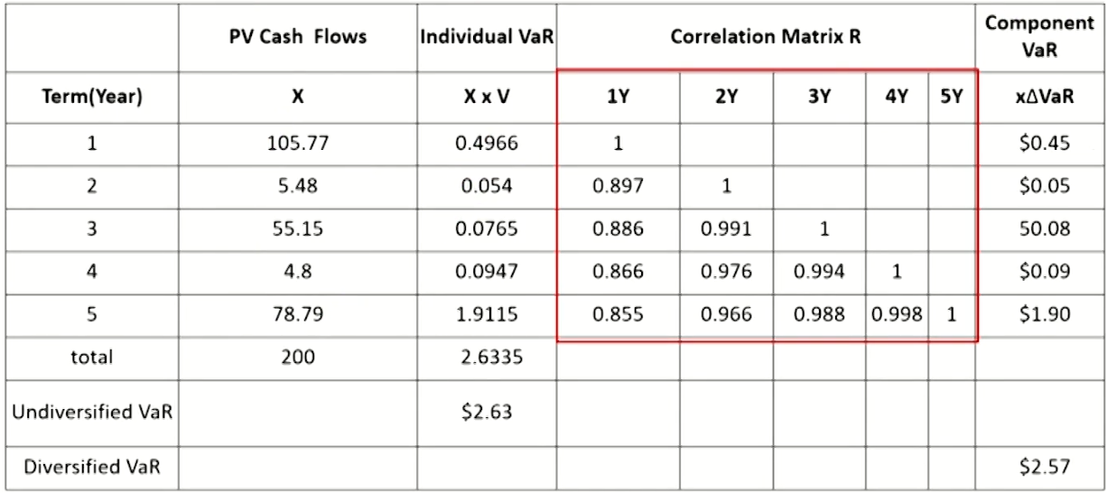
Performance Benchmarking
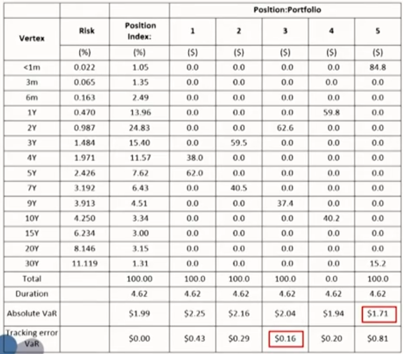
- Tracking error VaR: the VaR of the deviation between the target portfolio and the benchmark portfolio.
- Minimizing absolute market risk is not the same as minimizing relative market risk.最小化绝对市场风险不代表最小化相对市场风险
Mapping linear derivatives
- Since the value of linear derivatives is linear in the underlying,their risk can be constructed easily from basic building blocks.
- Mapping forward
- Mapping forward rate agreements (FRAs)
- Mapping interest-rate swaps
- Mapping forward
- Long foreign currency forward = long foreign currency spot + long foreign currency bill + short U.S.dollar bill
- Mapping forward rate agreements (FRAs)
- Long 6x12 FRA = long 6-month bill + short 12-month bill
This is equivalent to borrowing USD 100 million for 12 months and investing the proceeds(进项款) for 6 months - Short 6x12 FRA = short 6-month bill + long 12-month bill
This is equivalent to borrowing UsD 100 million for 6 months and investing the proceeds for 12 months
- Long 6x12 FRA = long 6-month bill + short 12-month bill
- Interest-rate swaps can be viewed in two different ways:
- A combined position in a fixed-rate bond and in a floating- rate bond.
A swap with receiving floating rate and paying fixed rate = long floating-rate bond + short fixed-rate bond - A portfolio of forward contracts.
- A combined position in a fixed-rate bond and in a floating- rate bond.
Mapping non-linear derivatives
- The BSM model can be applied to simplify the mapping of European options.
c=S_0N\left(d_1\right)-X e^{-r T} N\left(d_2\right)- Long call option = long \Delta asset + short (\Delta S-c) bill
- N\left(d_1\right)=\Delta
- X e^{-r T} N\left(d_2\right)=S N\left(d_1\right)-c=\Delta S-c
Correlations and Copulas
Correlation Basics: Definitions, Applications, and Terminology
Financial correlation risk
- Static financial correlations: measure how two or more financial assets are associated within a certain time period.
- Dynamic financial correlations: measure how two or more financial assets move together in time.
- Financial correlation risk: the risk of financial loss due to adverse movements in correlation between two or more variables.
Example of fihancial correlation risk
- An investor has invested $1 million in a bond from Spain, and purchased a CDS from a French bank, BNP Paribas(法国巴黎银行), because he is now worried about Spain defaulting.
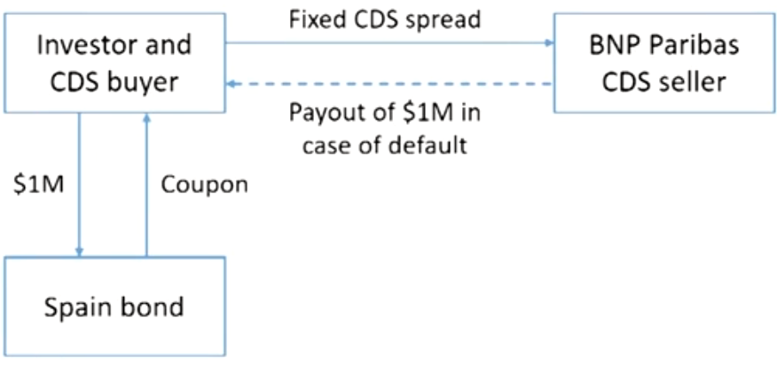
- CDS spreads of a hedged bond purchase with respect to the default correlation between the Spain bond and the BNP Paribas.
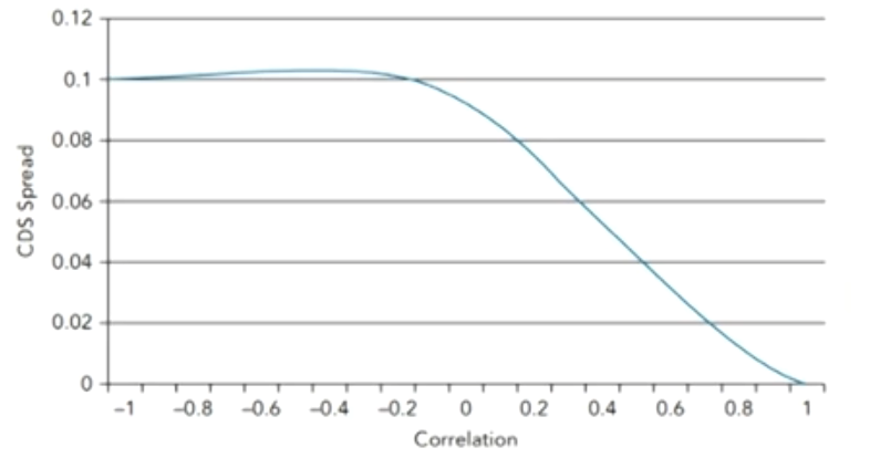
- If the correlation between Spain and BNP Paribas increases,the value of the CDS will decrease and the investor will suffer a paper loss(账面损失)
- If there is a positive default correlation between the two,the investor has wrong-way correlation risk(WWR).
Correlation in investment
- The return and risk for a portfolio with two assets:
\begin{gathered}R_p=w_1R_1+w_2R_2\\ \sigma_p=\sqrt{w_1^2\sigma_1^2+w_2^2\sigma_2^2+2w_1w_2\rho_{1,2} \sigma_1\sigma_2}\end{gathered}- Return/risk ratio: a risk-adjusted return for a portfolio. The higher, the better
Correlation in trading
- Generally, correlation trading means trading assets whose prices are determined at least in part by the co-movement of one or more asset in time
- Multi-Assets Options
- Quanto Options
- Correlation Swaps
- Multi-asset option (correlation option): the value of option is very sensitive to the correlation among multi-assets.
- Options on the better of two : payoff = Max(S1, S2)
- Options on the worse of two: payoff = Min(S, S2)
- Call on the Max. of two: payoff = Max[0, Max(S, S2)- K]
- Exchange option: payoff = Max(0, S2- S1)
- Spread call option: payoff = Max[0,(S,- S)-K]
- Quanto options(双币种期权):optionsthat allow a domestic investor to exchange his potential option payoff in a foreign currency back into his home currency at a fixed exchange rate.
- A quanto option therefore protects an investor against currency risk.
- The correlation between the price of the underlying (S) and the exchange rate (X) significantly influences the quanto call option price.
- The more positive the correlation coefficient,the lower the price for the quanto option.
- Correlation swap: a fixed (known) correlation is exchanged with the correlation that will actually occur, called realized or stochastic(unknown) correlation.
- The realized correlation \rho is calculated as:
\rho_{\text {realized }}=\frac{2}{n^2-n} \sum_{i>j} \rho_{i, j}
\rho_{i, j} : Pearson correlation between asset \mathrm{i} and \mathrm{j}
n : number of assets - The payoff of a correlation swap for the correlation fixed rate payer at maturity is:
\text{Payoff} = \text{Notional amount} \times\left(\rho_{\text {realized }}-\rho_{\text {fixed }}\right) - Another way of buying correlation (benefiting from an increase in correlation) is to buy call options on an index and sell call options on individual stocks of the index.
If correlation between the stocks of the index increases, so will the implied volatility of the call on the index.
This increase is expected to outperform the potential loss from the increase in the short call positions on the individual stocks.
- The realized correlation \rho is calculated as:
Correlation in market risk
- The equation for VaR for portfolio is:
- The VaR for the portfolio increases as the correlation among the assets in the portfolio increases.
V a R_p=\sqrt{x} \sigma_p \alpha
\sigma_p: the daily volatility of the portfolio, including the correlation among the assets
\alpha: the z-value from the standard normal distribution for a specific confidence level
x: the number of trading days
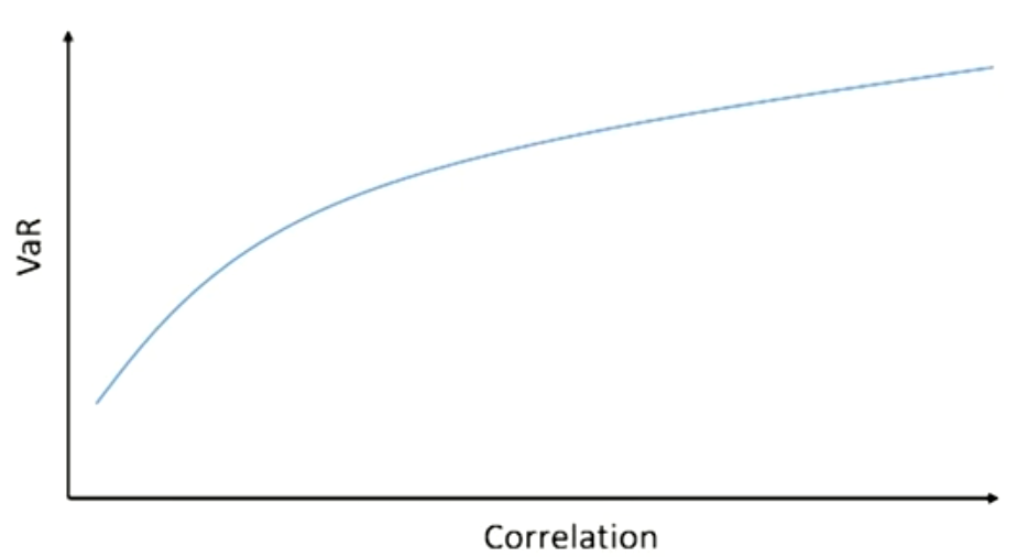
- The VaR for the portfolio increases as the correlation among the assets in the portfolio increases.
Correlation in credit risk
- According to the historical data, we observe that the default correlation within sectors is higher than between sectors.
- This suggests that macro systematic factors have a greater impact on defaults than do idiosyncratic factors.
- E.g., if General Motors defaults, it is more likely that Ford will default, rather than Ford benefiting from default of its rival.
- For most investment grade bonds, the term structure of default probabilities increases in time.
- The longer the time horizon, the higher the probability of adverse internal events.
- For bonds in distress, the term structure of default probabilities decreases in time.
- For a distressed company the immediate future is critical.If the company survives the coming problematic years,probability of default decreases.
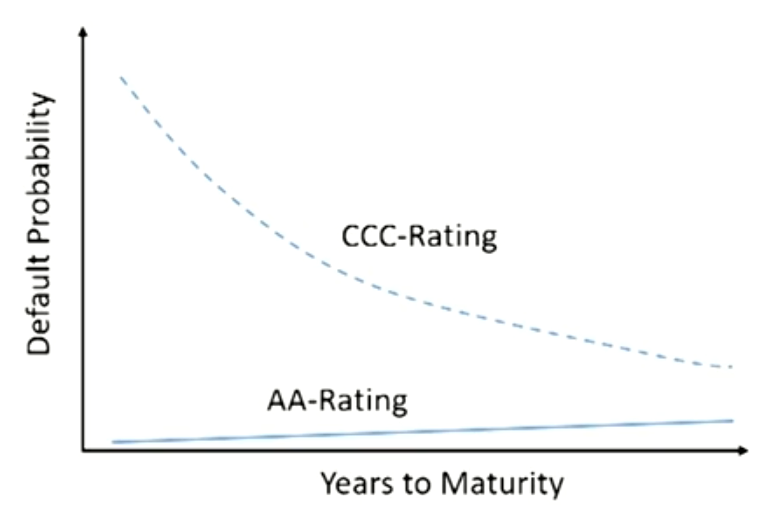
- For a distressed company the immediate future is critical.If the company survives the coming problematic years,probability of default decreases.
Correlation and systemic risk
- Systemic risk: the risk of a financial market or an entire financial system collapsing.
- Systemic risk and correlation risk are highly dependent.
- A systemic decline in stocks involves the entire stock market,correlations between the stocks increase sharply.
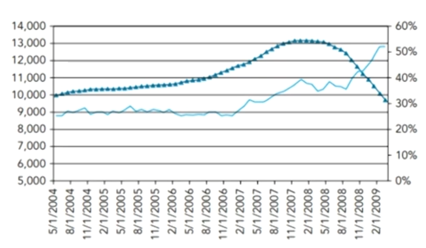
- A systemic decline in stocks involves the entire stock market,correlations between the stocks increase sharply.
Correlation and concentration risk
- Concentration risk: the risk of financial loss due to a concentrated exposure to a group of counterparties.
- Concentration risk can be quantified with concentration ratio.
- E.g., if creditor has 10 loans of equal size, the concentration ratio is 0.1.
- The lower the concentration ratio, the more diversified is the default risk of the creditor.
- In conclusion, the beneficial aspect of a lower concentration ratio is closely related to a lower correlation coefficient
- In particular, both a lower concentration ratio and a lower correlation coefficient reduce the worst-case scenario for a creditor, the joint probability of default of his debtors.
Correlation in the financial crisis
- From 2007 to 2009,default correlations of the mortgages(成分资产相关性)in the CDOs increased.
- The CDO equity tranche spread decreases and the value of the equity tranche increases.
- However, this increase was overcompensated by a strong increase in default probability of the mortgages.
Tranche spreads increased sharply, resulting in huge losses for the equity tranche investors as well as investors in the other tranches.
- Correlations between the tranches(层级间相关性)of the CDOs also increased during the crisis. This had a devastating effect on the super-senior tranches.
- In normal times, these tranches were considered extremely safe, but with the increased tranche correlation and the generally deteriorating credit market, these super-senior tranches were suddenly considered risky and lost up to 20%of their value.
Empirical Properties of Correlation
Correlation and correlation volatility
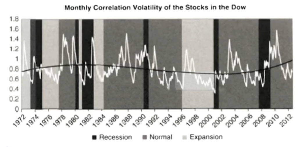
- In our study, we observed daily closing prices of the 30 stocks in the Dow Jones Industrial Average (Dow) from January 1972 to July 2017, applying the Pearson correlation approach.

- Correlation levels are lowest in strong economic growth times and typically increase in recessions.经济扩张时高,衰退时低
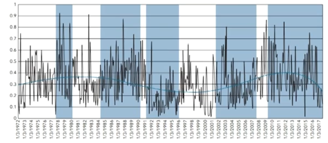
- Correlation volatility is lowest in an economic expansion and highest in normal economic states.经济正常时高,扩张时低
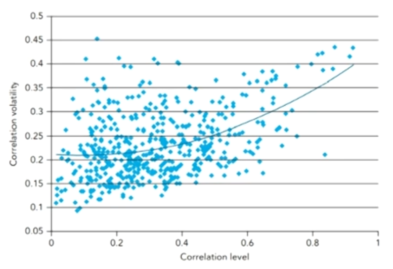
- There is a positive relationship between correlation level and correlation volatility.
- Correlation levels are lowest in strong economic growth times and typically increase in recessions.经济扩张时高,衰退时低
- Mean reversion(均值复归): the tendency of a variable to be pulled back to its long-term mean.
- Mean reversion is present if there is a negative relationship between S_t-S_{t-1} and S_{t-1}。
- Many variables such as interest rates, volatilities, credit spreads are assumed to exhibit mean reversion
- Formula for mean reversion:
S_t-S_{t-1}=a\left(\mu_S-S_{t-1}\right) \Delta t+\sigma_S \varepsilon \sqrt{\Delta t}
S_t: price at time t; S_{t-1}: price at the previous point in time。
a: Mean reversion rate, 0\leq a \leq1。
\mu_S : long term mean of \mathrm{S} ; \sigma_S : volatility of \mathrm{S}。
\varepsilon : random drawing from standardized normal distribution。
\sigma_S \varepsilon \sqrt{\Delta t} : the stochasticity part。 - By ignoring the stochasticity part and assuming \Delta \mathrm{t}=1 :
S_t-S_{t-1}=a\left(\mu_S-S_{t-1}\right)=a \mu_S-a S_{t-1} - To find the mean reversion rate a, we can run a standard regression analysis of the form:
\begin{aligned} & \quad S_t-S_{t-1}=a \mu_S-a S_{t-1} \Rightarrow Y=\alpha+\beta X \\ & Y: S_t-S_{t-1} \\ & X: S_{t-1} \\ & \alpha: a \mu_S \\ & \beta:-a\end{aligned}
Autocorrelation
- Autocorrelation (AC): the degree to which a variable is correlated to its past values. The autocorrelation (AC) for a one-period lag is defined as:
A C\left(\rho_t, \rho_{t-1}\right)=\frac{\operatorname{Cov}\left(\rho_t, \rho_{t-1}\right)}{\sigma\left(\rho_t\right) \sigma\left(\rho_{t-1}\right)}- 1-period autocorrelation + mean reversion rate = 1
- Autocorrelation is the "reverse property" to mean reversion: the stronger the mean reversion, the lower the autocorrelation, and vice versa.
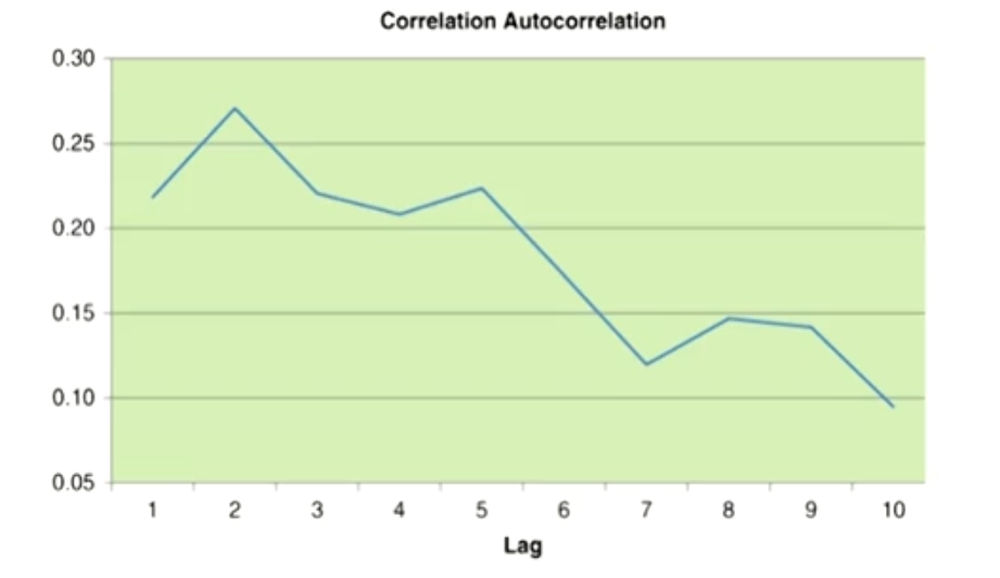
- The highest autocorrelation was found using a two-day lag,and autocorrelations decay with longer time period lags.总体下降,最大值在两期
Best-fit distributions for correlations
- Equity correlation: the Johnson SB distribution provides the best fit. Standard distributions such as normal distribution,lognormal distribution provided a poor fit.
- Bond correlation: best fitted with the generalized extreme value (GEV) distribution and quite well with the normal distribution.
- Default probability correlation: the Johnson SB distribution.
Financial Correlation Modeling: Bottom-Up Approaches
Copula functions
- Copula functions allow the joining of multiple univariate distributions (marginal distributions) to a single multivariate distribution
- Transform two or more unknown distributions and mapping them to known distributions with well-defined properties.
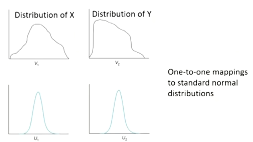
- Gaussian copula maps each unknown variable distribution (marginal distribution) to the standard normal distribution.未知的分布映射为已知分布
- The rule for the mapping is percentile-to-percentile basis.
Gaussian copula
- Graphical representation of the copula mapping N^{-1}(Q(t))
- Gaussian copula model
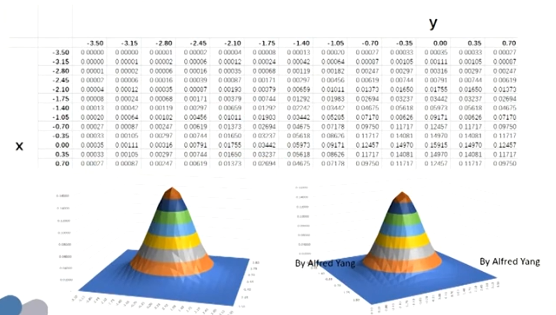
- David Li (2000) transferred the copula function to finance (valuing CDOs)。 He defined cumulative default probabilities Q for entity i at a fixed time t, Q_i(t) as marginal distributions。Then the Gaussian default time copula \left(C_{G D}\right) :
C_{G D}\left[Q_1(t), \ldots, Q_n(t)\right]=M_n\left\{N^{-1}\left[Q_1(t)\right], \ldots, N^{-1}\left[Q_n(t)\right] ; \rho_M\right\}
- David Li (2000) transferred the copula function to finance (valuing CDOs)。 He defined cumulative default probabilities Q for entity i at a fixed time t, Q_i(t) as marginal distributions。Then the Gaussian default time copula \left(C_{G D}\right) :
Term structure models of interest rates
The Science
Risk-neutral pricing
- Problems: Expected discounted value is not the same as market value.
- Solution: take the rates on the tree as given and adjust the probabilities so that the expected discounted value from the model is equal to its current market price.
- Use risk-neutral probabilities, other than assumed true or real-world probabilities for the up and low-path.
- The difference between true and risk neutral probabilities is described in terms of the drift in interest rates.
- Under the assumed true probabilities, the drift of the six-month rate, or the expected change in the six- month rate, is zero.
- Under the risk-neutral probabilities, the drift of the six-month rate is 30.24 basis points.
Issues with interest rate tree model
- Recombining tree vs.non-recombining tree节点不重合
- More economic and reasonable non-recombining trees but difficult to implement: N+1 possible states for recombining trees but 2^N possible states for non-recombining trees. Size of time steps
- Smaller time step generates more realistic interest rate distributions, but poses numerical issues like round-off error and increases computation time.
- BSM model does not apply to bond options:
- The model assumes that the price of stock follows a random process, but bond price converges to face value at maturity.
- The model assumes that volatility of stock price is constant,but volatility of bond price gets smaller as time extends.
- The model assumes the short-term interest rate is constant,but this assumption obviously does not work for pricing analysis of bond option.
The Evolution and Shape
The shape of the term structure
- Spot or forward rates are determined by:
- Expectations of future short-term rates (without any uncertainty)
- Volatility of short-term rates(with any uncertainty but under the assumption of risk-neutrality)
- Interest rate risk premium (with the assumption of risk-averse)
- Jensen's inequality
E\left[\frac{1}{1+r}\right]>\frac{1}{E[1+r]}=\frac{1}{1+E[r]}- Introducing volatility, yield is reduced by convexity.
- Convexity is related to
- Maturity: convexity increase with maturity
- Yield: convexity lowers bond yields
- Volatility: convexity increases with volatility
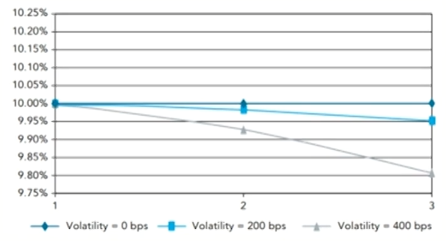
Risk premium
- Assuming investors demand an extra 20 basis points for each year of interest rate risk, the price of the two-year zero is:
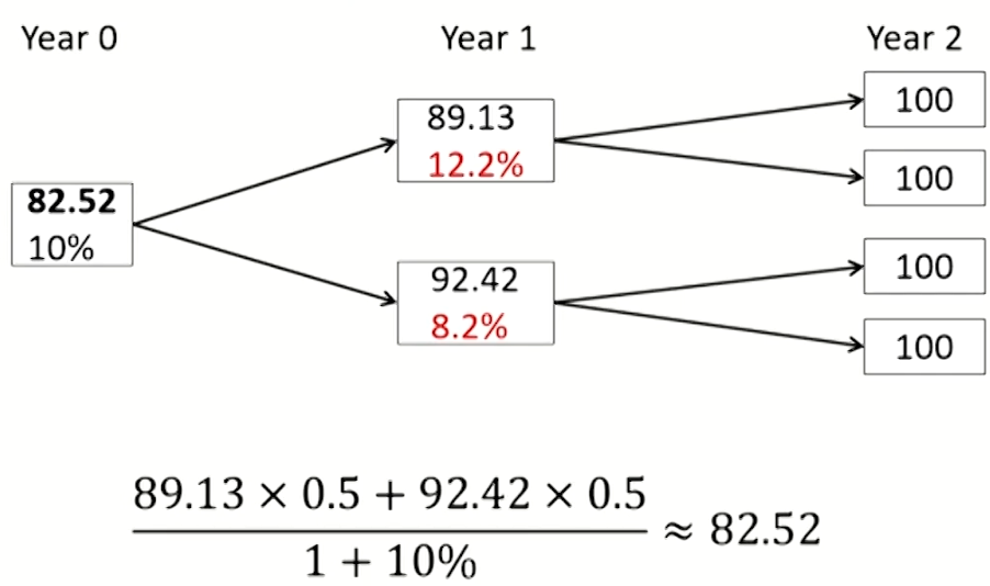
- In case of no risk premium, the term structure of spot rates is downward-sloping due to convexity.
- In case of modest risk premium:
- In the short end, the risk premium effect dominates and the term structure is mildly upward-sloping.
- In the long end, the convexity effect dominates and the term structure is mildly downward-sloping.
- In case of large risk premium, risk premium dominates the convexity and term structure of spot rates is upward-sloping.
Term Structure Models
Models with Drift
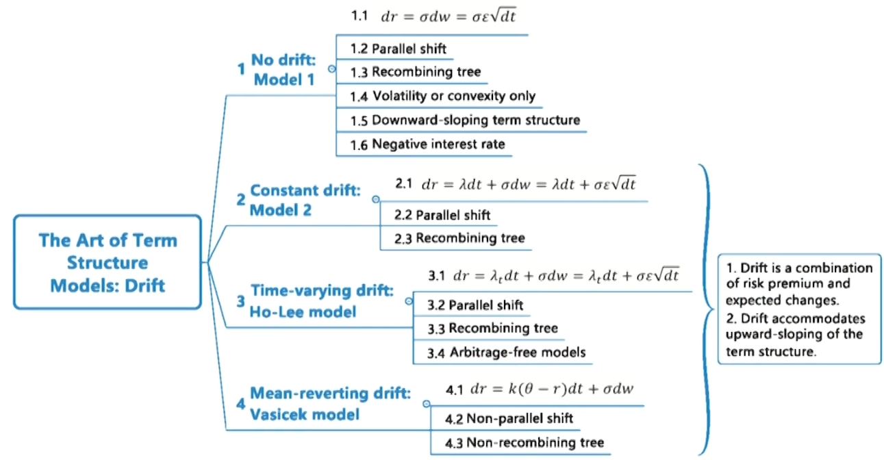
Model 1
- A problem with model 1 is that the short-term rate can become negative. Solutions include:
- Changing the distribution of interest rates, such as lognormal distribution.
- Simply set all negative rates to zero.
Vasicek model
- Problem: this tree does not recombine since the drift increases with the difference between the short-term interest rate and 0.
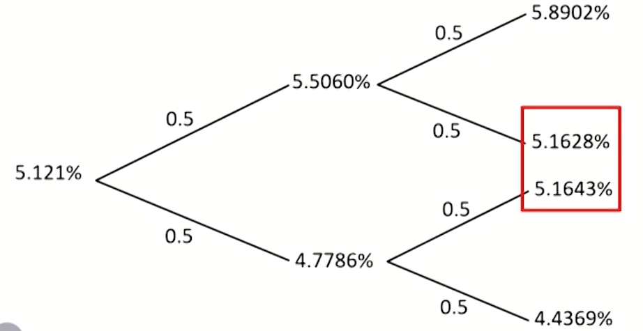
- Solution:
- 平均值合成节点,然后更新概率
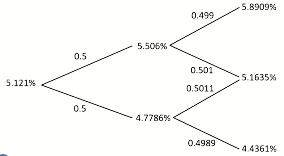
- 平均值合成节点,然后更新概率
- Some important conclusions:
- The model applies expected interest rates and standard deviations to solve the probabilities of up and down states.根据期望值和标准差更新概率
- In creating recombining trees, probabilities of up or down states must not be necessarily equal at different nodes.更新后概率不一定相同
- Volatilities after T years
- For models without mean reversion, the standard deviation of the terminal distribution after T years increases with the square root of time.
- For Vasicek model with mean reversion, the standard deviation after T years increases with horizon more slowly.
- Annualized volatilities
- For Vasicek model, the volatilities decline with term, and the impact of convexity is also lower.第一项递减,第二项恒定
- For model 1, model 2 and Ho-Lee model, the term structure of volatility is constant or flat, and fails to capture the volatility structure in the market.
- The term structure of volatility in the market is humped驼峰状: initially rises with term but eventually declines.
- The expectation of rate in the Vasicek model after T years is:
r_0e^{-k T}+\theta\left(1-e^{-k T}\right)- \theta: long-term equilibrium interest rate
- k: the speed of mean reversion
- The half-life :The time it takes the factor to progress half the distance toward its goal.
\tau=\frac{\ln2}{k}
Models with Volatility and Distribution
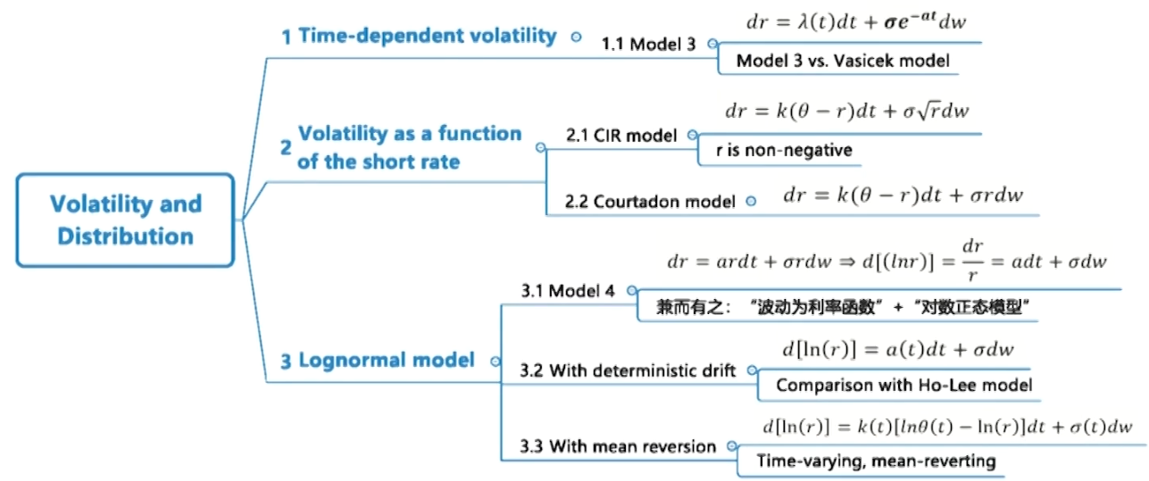
Model 3 vs. Vasicek model
- Annualized volatilities
- For Vasicek model, the volatilities decline with term, and the impact of convexity is also lower.
- For model 3, The volatility starts at the constant σ and then exponentially declines to zero.
- T-year volatilities
- For both Vasicek model and model 3, the standard deviation increases with horizon more slowly.
- The behavior of standard deviation as a function of horizon for model 3 resembles the impact of Vasicek model.
- Setting the initial volatility and decay rate (a) in Model 3equal to the volatility and mean reversion rate (k) of the Vasicek model, the standard deviations of the terminal distributions from the two models turn out to be identical.
- Model 3 is a parallel shift model. While Vasicek model implies nonparallel shift model.
- Different purposes favor different models:
- If the purpose is to quote fixed income options prices that are not easily observable, Model 3 is more feasible.
- If the purpose is to value and hedge fixed income securities, a model with mean reversion might be preferred.
CIR model,Courtadon model and model 4
- Three models have improvements over models with constant basis-point volatility that allows r to be negative.
- \sigma: yield volatility, which is constant.
- \sigma r or \sigma \sqrt{r}: basis-point volatility.
- \sigma r increases with r linearly.
- \sigma \sqrt{r} is proportional to the square root of rate, implying basis point volatility increases with r at a decreasing rate.
Lognormal model vs.Normal model
- Normal model: The short rate is normally distributed.
- Lognormal model :The natural logarithm of the short rate is normally distributed, which implies that the short rate is lognormally distributed. Lognormal model vs. Ho-Lee model
- In the Ho-Lee model the drift terms are additive, but in the lognormal model with deterministic drift, the drift terms are multiplicative
Other related topics
Academic Literature of the Trading Book
VaR, expected shortfall and spectral risk measures
- Value at Risk(VaR) has become a standard risk measure in finance due to its conceptual simplicity, computational facility,and ready applicability, but:
- VaR measures only quantiles of losses, and thus disregards any loss beyond
- It has been criticized for its lack of subadditivity, leading to not being a coherent risk measure (Subadditivity, Positive homogeneity, Monotonicity, Transition property).
- Expected shortfall (ES) has the following properties:
- ES accounts for the severity of losses beyond the confidence threshold and it is always subadditive and coherent.
- VaR can't ensure estimate of portfolio risk is less than or equal to the sum of risks of portfolio's positions, ES does.次可加性
- It mitigates the impact that the particular choice of a single confidence level may have.
- Backtesting ES is more complicated and less powerful than backtesting VaR.不够强力
- Spectral (谱) risk measures(SRM) are a generalization of ES. SRM requires little effort if the underlying risk model is simulations-based. SRM has advantages over ES, including:
- Favorable smoothness and the possibility of adapting the risk measure directly to the risk aversion of investors.
- SRM is not bound to a single confidence level compared with ES or VaR.
Fundamental Review of the Trading Book
Internal models-based approaches
- Basel I and Basel II.5: based on VaR for a 10-day horizon with a 99% confidence level.
- FRTB: based on stressed expected shortfall(ES) with five liquidity horizons and with a 97.5% confidence level
- It typically uses historical simulation method to estimate ES.
- Five different liquidity horizons: 10 days, 20 days, 40 days,60 days, and 120 days.
- Banks can not determine liquidity horizon for market variables but count upon guidance from Basel framework. and Basel II.5: based on VaR for a 10-day horizon with a 99%confidence level.
- If losses have a normal distribution that has a mean u and standard deviation σ, 99% VaR is μ + 2.326σ, 97.5% ES is μ + 2.338σ, the two measures are almost σ.
- For non-normal distributions, they are not equivalent. When loss distribution has a heavier tail than normal distribution,97.5% ES can be considerably greater than 99% VaR.
- Credit risk:
- Credit spread risk: the risk that credit spread changes causing the mark-to-market value of the instrument to change. It handled in a similar way to other market risks.
- Jump-to-default risk多家违约: the risk that there will be a default by the company. It is handled in the same way as default risks in the banking book based on VaR calculation with one year time horizon and 99.9% confidence level.
- Back-testing: FRTB does not back-test the stressed ES measures but back-tests a bank's models by asking each trading desk to back-test a VaR measure calculated over a one-day horizon and the most recent 12 months of data.
- Both 99% and 97.5% confidence levels are to be used.
- If more than 12 exceptions for 99% VaR or more than 30 exceptions for 97.5% VaR, the trading desk is required to calculate capital using the standardized approach until neither of these two conditions continues to exist.
Standardized Approach
- The capital requirement is the sum of three components:
- A risk charge calculated using a risk sensitivity approach
- A default risk charge: It refers to as jump-to-default(JTD) risk
- A due residual risk add-on: It includes exotic options when they cannot be considered as linear combinations of plain vanilla options.
- A risk charge calculated using a risk sensitivity approach. Seven risk classes (corresponding to trading desks)
- General interest rate risk, foreign exchange risk,commodity risk, equity risk, three categories of credit spread risk.
- Within each risk class, a delta risk charge, vega risk charge, curvature risk charge are calculated.
Other important conclusions
- The standardized approach to provide a floor for capital requirements must be used even if a bank is approved to use an internal models approach.
- FRTB further counteracts regulatory arbitrage to present less subjectivity and flexibility by defining more clearly and providing rules for different positions in determining whether they should be placed in trading book or banking book
- Basel I and Basel ll.5 required that market risk be calculated on a firm-wide basis, while FRTB allowed market risk to be calculated at the trading desk level. Permission to use the internal models approach is granted on a desk-by-desk basis.
- It is possible that a bank's foreign currency trading desk has permission to use the internal models approach while the equity trading desk does not.
Empirical Approaches to Risk Metrics and Hedges
DV01-neutral hedge
- DV01: the change of bond price in currency unit when its yield changes by one basis point.
- DV01-neutral hedge: the hedged portfolio has the same DV01 with hedging instrument, so the offsetting make the DV01 of the entire position equal zero.
- This hedge ensures that if the yield on the hedged portfolio and the hedging instrument both increase or decrease by the same number of basis points, the trade will neither make nor lose money.
Single-variable regression-based hedging
- The hedge coefficient (\beta) can be obtained by regression:
\Delta r_t^\text{T-bond}=\alpha+\beta \Delta r_t^{\text {TIPS }}+\varepsilon_t- \Delta r_t^{\text {T-bond }} : changes of the yield for $T$-bond.
- \Delta r_t^{\text {TIPS }} : changes of the yield for TIPS.
- Hedge coefficient or hedge adjustment factor (\beta) : the ratio of the average yield change for hedged portfolio to that for the hedging instrument.
Volatility Smiles
Volatility smile for foreign currency options
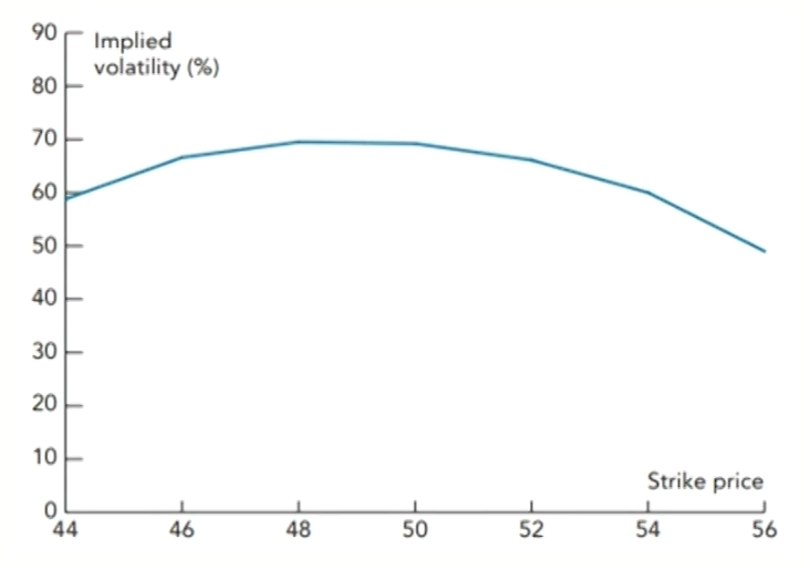
- The implied volatility is relatively low for at-the-money (ATM) options. It becomes progressively higher as an option moves either to in-the-money(ITM) or out-of-the-money(0TM).
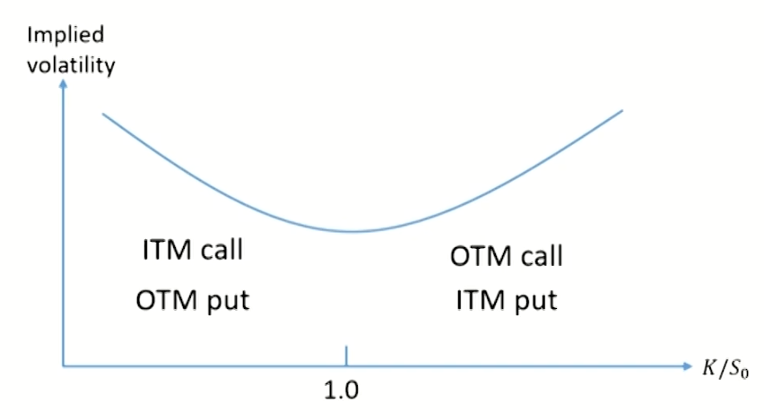
- Implied distribution: the risk-neutral probability distribution for an asset price at a future time from the volatility smile given by options maturing at that time.
- For foreign currency options, the implied distribution has heavier tails (higher kurtosis) than the lognormal
- distribution with the same mean and standard deviation.It is consistent with the implied volatility for foreign currency option.
- Implied distribution causes the volatility smile.
- Implied distribution has more observations around the mean and more observations in both tails.
Volatility smile for equity options
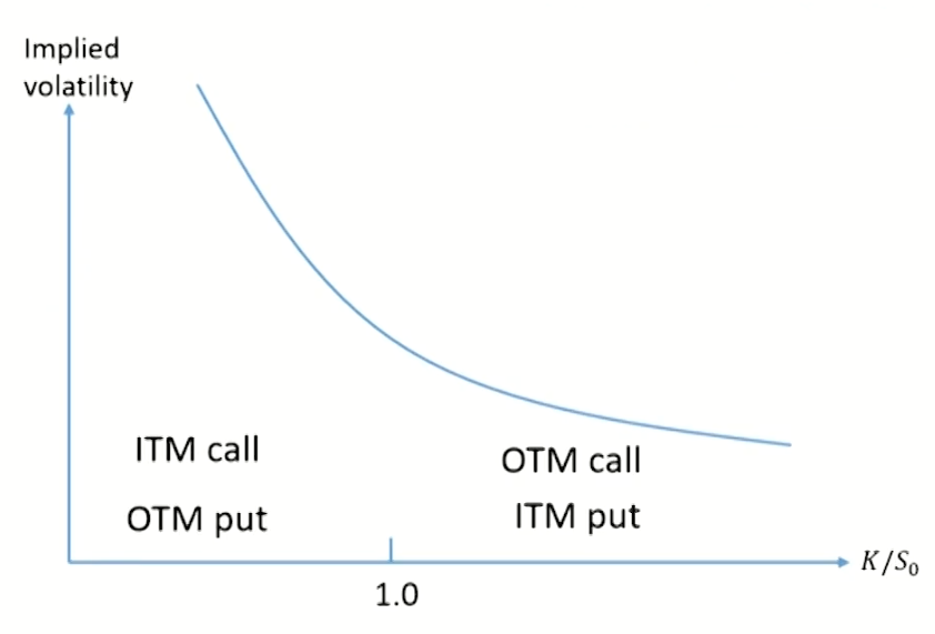
- The implied volatility decreases as the strike price increase:
- Sometimes referred to as a volatility skew(or smirk).
- The volatility used to price a low-strike-price option is significantly higher than that used to price a high-strike-price option.
- The implied distribution has a heavier left tail and a less heavy right tail than the lognormal distribution with the same mean and standard deviation.
- There is a negative correlation between equity prices and volatility, and there are several possible reasons for this:
- Leverage effect: as equity prices move down/up, leverage increases/decreases and as a result volatility increases/decreases.
- Volatility feedback effect: as volatility increases/decreases,investors require a higher/lower return and as a result the stock price declines/increases.
- Crashophobia(崩盘效应)
Volatility surface
- Combine volatility smiles with the volatility term structure to tabulate the volatilities appropriate for pricing an option with any strike price and any maturity.
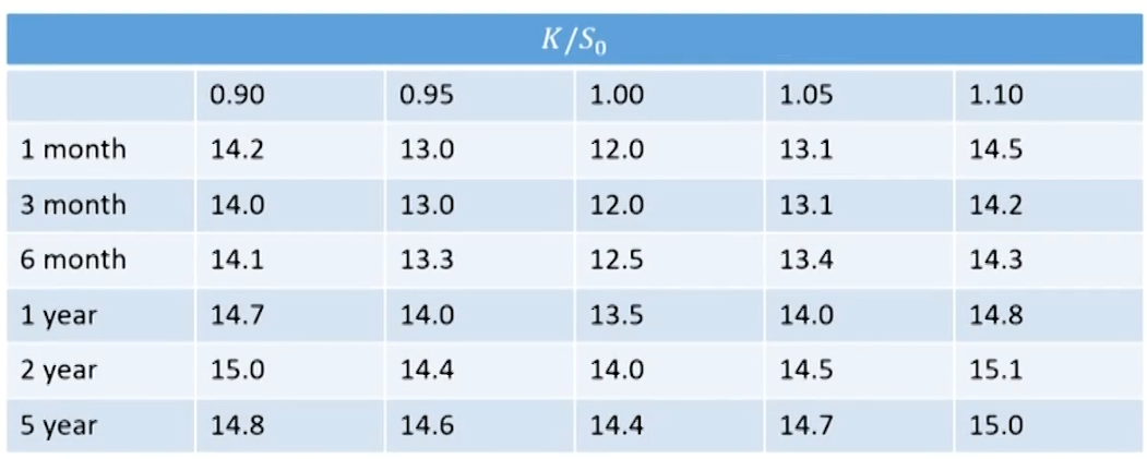
- Conclusion: The shape of the volatility smile depends on the option maturity. The smile tends to become less pronounced as the option maturity increases, i.e.the smile curve presents a steep shape with short-term maturities but a flat shape with long-term maturities.
Impact of price jump
- The probability distribution of the stock price (large jumps) in the future might then consist of a mixture of two lognormal distributions, the first corresponding to favorable news, the second to unfavorable news.

- It is actually a "frown" with volatilities declining as we move out of or into the money.
